 Miscellanies: simple calculator for paleomagnetism; pcalc
Program "pcalc" provides an interactive utility in which manual calculations of paleomagnetic data are possible as a simple calculator. To use it, type "pcalc" with "-A" option which stands for "assorted". When table of items is displayed, type the item number which you want to do.
Example of Fisher statistics
The next snapshot illustrates Fisher statistics of eight sample directions by selecting "Item 7".
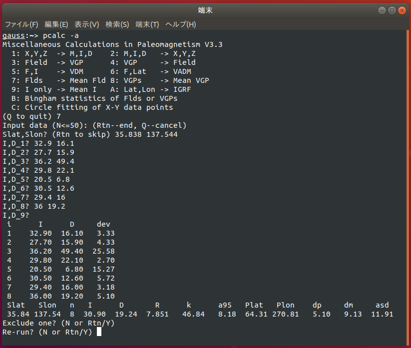
The program asks you if you wish to exclude one datum from the statistics. However, this function is not to encourage you to eliminate an inconvenient datum arbitrary. You should carry out the statistical test of outlier (McFadden, 1982) which is available by the program "tmeandir".
Case of Bingham statistics
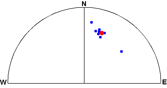
The above input data used for "Item 7" are quite elongated as shown in the figure, possibly due to failed elimination of the secondary remanence components. Selecting "Item B" (Bingham statistics of Flds or VGPs) and supplying the same data, the following results are displayed together with Fisher statistics at the last (first a cautionary message appears, but just hit "Return" key to continue).
Bingham statistics:
  n     k1     k2     tau1   tau2   tau3
  8  -214.49 -15.43   0.02   0.27   7.71
  I3(Lat3) D3(Lon3)  I2(Lat2) D2(Lon2)  I1(Lat1) D1(Lon1)
     30.83   18.95     21.51  122.56     50.93  241.61
  a31    a32    a21     Xu     Xcp     Xcg
  2.44   9.25  14.04   35.83   24.93   57.41
Fisher statistics:
  n Im(Latm) Dm(Lonm)   R       k     a95    Asd
  8   30.90   19.24    7.85   46.84   8.18  11.91
Among parameters displayed above, the direction of eigenvector \({\bf t}_3\) is shown under the head "I3(Lat3) D3(Lon3)". This is in excellent agreement with the mean direction of Fisher statistics obtained in "Item 7" (or, those shown under the head "Im(Latm) Dm(Lonm)"). However, Bingham statistics revealed that there is a large elongation in the 95% confidence region because \(\alpha_{32}\) is much larger than \(\alpha_{31}\) (shown under the head "a31 a32").
Main field elements from IGRF
"Item A" provides calculation of the main field elements from IGRF-14 for the time span AD 1900--2029 with summation up to n=13 (AD 2000 and later) or n=10 (before AD 2000).
Geomagnetic elements from IGRF-14.
  ** Maximum n is 13 for year >= 2000, and n is 10 for year < 2000. **
  ** Geodetic coordinate system WGS-84 (lat,lon) & altitude = 0 km. **
  ** Give the date in decimal year (ex.: 2025.3315 for 1 May 2025)  **
  ** For more options such as geocentric system, use program "igrf" **
Continue? (Rtn or Y/N)
Decimal year? 2025.2
Year: 2025.20
Slat,Slon? -40.3 175.7
 Slat    Slon  F(nT)   I      D
-40.30  175.70 55008 -65.49  22.61
Slat,Slon?
If field elements at a certain altitude or in geocentric coordinates are necessary, use another program "igrf".
Circle fitting
A unique function to "pcalc" is circle fitting of 2-dimensional X-Y data by Taubin method. Though this was originally aimed for use in analyzing paleointensity data, it can be applied to general data as the next example. Select "Item C" and input four points, the results are as below.
Input X-Y data (3<=N<=50)
X,Y_1? 1.1 0.0
X,Y_2? 0.0 0.9
X,Y_3? -1.1 0.0
X,Y_4? 0.0 -0.9
X,Y_5?
 i     X         Y         Error
 1    1.100     0.000     0.09501
 2    0.000     0.9000   -0.1050
 3   -1.100     0.000     0.09501
 4    0.000    -0.9000   -0.1050
 N   X0        Y0        R         k         SSE
 4  0.000     0.000     1.005     0.000     0.04010
Exclude one? (N or Rtn/Y)
"(X0,Y0)" and "R" are the center and the radius of the fitted circle, respectively. Note that the radius R is slightly larger than the optimal value of 1. This is because the program minimizes sum of the squares of the "algebraic" distance "\(r_i^2 - R^2\)", not that of the "geometric" distance "\(r_i - R\)", where \(r_i\) is the distance of a data point from the center. Although the algebraic fits are less accurate than the geometric fits, the former algorithm is simpler and hence widely used. For the details of the theory, see Chernov & Lesort (2005). "k" and "SSE" are a measure of the curvature and sum of the squares of the Error which is \(r_i-R\), respectively. They are used to evaluate the paleointensity data, and hence can be ignored for general data (see "MEMOS_PMAGT402.pdf" contained in "pmagt402.tar.gz").
Data input from a file
"pcalc" also reads input data from a file by using options other than "-A". In this case, the number of input data is limitless but the interactive function such as excluding an outlier is not available. Hence, with such options you can redirect the results to a file (but do not redirect with option "-A"!). The following example of option "-I" shows inclination only statistics which are read from "t-inc.d". "-L" option is also used to list the input data.
pcalc -i -l t-inc.d > result.txt
The content of the output file "result.txt" is as the followings.
Inclination only statistics of t-inc.d:
Arith. mean: Im= 68.78, km= 36.42
MLE estimations:
 n   Im      km     a95   iteration
 9  71.85   32.45   9.17      43
Input data:
 i    I     dev
 1  66.10  -5.75
 2  68.70  -3.15
 3  70.10  -1.75
 4  82.10  10.25
 5  79.50   7.65
 6  73.00   1.15
 7  69.30  -2.55
 8  58.80 -13.05
 9  51.40 -20.45
In this case, convergence of the process was quite rapid after 43 iterations. Depending on the data, however, the convergence might be bad and in that case a cautionary message is displayed.
Download and installation of the program
Supplementary notes
VGP to Field direction
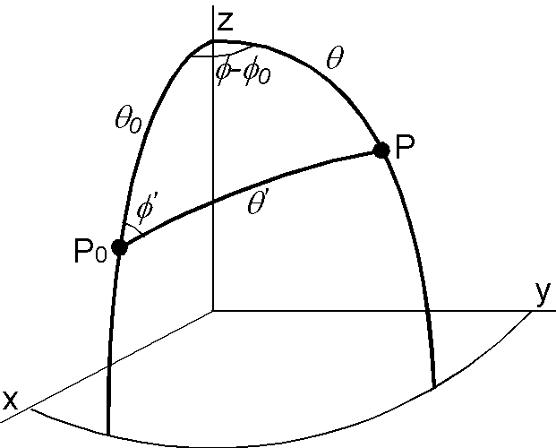
Given a VGP position \((\lambda_P,\phi_P)\), the field direction \((I,D)\) observed at a site \((\lambda_S,\phi_S)\) is obtained by using the spherical trigonometry which is converse of the formula for field to VGP. However, "pcalc" uses the relation of the geocentric dipole and the degree 1 Gauss coefficients. Considering that a VGP is actually a south pole, we have to use an inverted pole position \((-\lambda_P,\phi_P-180)\) to estimate the Gauss coefficients as \begin{eqnarray*} g_1^0 & = & \frac{\mu_0 M}{4\pi a^3}\sin(-\lambda_P) = -\frac{\mu_0 M}{4\pi a^3}\sin\lambda_P, \\ g_1^1 & = & \frac{\mu_0 M}{4\pi a^3}\cos(-\lambda_P)\cos(\phi_P-\pi) = -\frac{\mu_0 M}{4\pi a^3}\cos\lambda_P\cos\phi_P, \\ h_1^1 & = & \frac{\mu_0 M}{4\pi a^3}\cos(-\lambda_P)\sin(\phi_P-\pi) = -\frac{\mu_0 M}{4\pi a^3}\cos\lambda_P\sin\phi_P, \end{eqnarray*} where \(\mu_0\), \(M\), and \(a\) are permeability of free space, dipole moment, and the earth's radius, respectively. Using the geomagnetic potential of degree 1, the field components \(X\), \(Y\), \(Z\) (NS, EW, vertical, respectively) are given by \begin{eqnarray*} X & = & -g_1^0\sin\theta_S + (g_1^1\cos\phi_S + h_1^1\sin\phi_S)\cos\theta_S, \\ Y & = & g_1^1\sin\phi_S - h_1^1\cos\phi_S, \\ Z & = & -2 g_1^0\cos\theta_S - 2(g_1^1\cos\phi_S + h_1^1\sin\phi_S)\sin\theta_S, \end{eqnarray*} where \(\theta_S=90-\lambda_S\).
Fisher statistics
Bingham statistics
Inclination only statistics
Statistics of inclination only data was introduced to paleomagnetism in 1960's to analyze the paleomagnetic measurements from borecores which usually lack declinations. The first study which can be used as a computer algorithm was presented by Kono (1980). Among quite a few studies which followed, the method by McFadden & Reid (1982) has been the most used in the community. However, "pcalc" adopted the recent method of Arason & Levi (2010). The followings are concise introduction to the inclination only statistics.
Using polar coordinates, consider a direction P(\(\theta\),\(\phi\)) which is Fisher distributed around the true direction P\(_0\)(\(\theta_0\),\(\phi_0\)). Let \(\theta^\prime\) and \(\phi^\prime\) be the polar angle of P from P\(_0\) and the azimuthal angle of P around P\(_0\), respectively. The probability density function of P around P\(_0\) is given by \[ f(\theta^\prime,\phi^\prime)d\theta^\prime d\phi^\prime = {\scriptsize \frac{\kappa}{4\pi\sinh\kappa} }\exp(\kappa\cos\theta^\prime)\sin\theta^\prime d\theta^\prime d\phi^\prime. \] Using the spherical trigonometry (formulas are → here), the probability density is expressed in \((\theta,\phi)\) as \[ f(\theta,\phi)d\theta d\phi = {\scriptsize \frac{\kappa}{4\pi\sinh\kappa} }\exp[\kappa\cos\theta_0\cos\theta + \kappa\sin\theta_0\sin\theta\cos(\phi-\phi_0)]\sin\theta d\theta d\phi. \] Integrating this equation by \(\phi\), the density of the marginal distribution of \(\theta\), i.e. the probability density of \(\theta\) when \(\phi\) is unknown, is obtained as \[ f(\theta)d\theta = {\scriptsize \frac{\kappa}{2\sinh\kappa} }\exp(\kappa\cos\theta_0\cos\theta)I_0(\kappa\sin\theta_0\sin\theta)\sin\theta d\theta, \] where \(I_0(\cdot)\) is the modified Bessel function of the first kind of order 0. When \(N\) colatitudes \(\theta_i\) (\(i=1\cdots N\)) are given, the maximum likelihood estimations of \(\theta_0\) and \(\kappa\) are obtained by maximizing the following log-likelihood function \begin{eqnarray*} h(\theta,\kappa) & = & \log\prod_{i=1}^N f(\theta_i), \\ & = & N\log\left({\scriptsize \frac{\kappa}{2\sinh\kappa} }\right) + \sum_{i=1}^N\log(\sin\theta_i) + \sum_{i=1}^N\kappa\cos\theta_0\cos\theta_i \\ & & + \sum_{i=1}^N\log(I_0(\kappa\sin\theta_0\sin\theta_i)). \end{eqnarray*}
Differences of the studies published so far are in the methods of approximating the above equation, especially the Bessel function part. Here, it is presumed that the most reliable study is Arason & Levi (2010) in which detailed description was presented together with thorough comparison of the results among the previous studies.
International Geomagnetic Reference Field
Circle fitting
References:
- Arason, P., and S. Levi, Maximum likelihood solution for inclination-only data in paleomagnetism, Geophys. J. Int., 182, 753-771, 2010.
- Chernov, N., and C. Lesort, Least squares fitting of circles, J. Math. Imaging Vision, 23, 239-251, 2005.
- IAGA Working Group V-MOD, International Geomagnetic Reference Field: IGRF-13 is released, 2020. (URL: https://www.ngdc.noaa.gov/IAGA/vmod/igrf.html)
- Kono, M., Statistics of paleomagnetic inclination data, J. Geophys. Res., 85, 3878-3882, 1980.
- McFadden, P. L., Rejection of paleomagnetic observation, Earth Planet. Sci. Lett., 61, 392-395, 1982.
- McFadden, P. L., and A. B. Reid, Analysis of palaeomagnetic inclination data, Geophys. J. R. astr. Soc., 69, 307-319, 1982.