Fisher distribution
Paleomagnetic direction is determined from several measurements of remanence directions which have some dispersion. Statistics to analyze these remanence directions was developed by Fisher (1953). The probability density of an observation on the unit sphere is given by,
\begin{equation}
f(\theta) = \frac{\kappa}{4 \pi \sinh \kappa} e^{\kappa \cos \theta} \label{eq01}
\end{equation}
where \(\theta\) is an angle from the true direction and \(\kappa\) is the precision parameter, varying from 0 (uniform distribution) to \(+\infty\) (concentrated to a single point). The term \(\kappa/4\pi\sinh\kappa\) is a normalization factor. In fact, integrating \eqref{eq01} over the surface of the unit sphere,
 \begin{eqnarray*}
& & \int_0^{2\pi} \int_0^\pi \frac{\kappa}{4 \pi \sinh \kappa} e^{\kappa \cos \theta} \sin \theta d\theta d\varphi \\
& & = \frac{\kappa}{2\sinh \kappa}\left[-\frac{1}{\kappa}e^{\kappa \cos\theta}\right]_0^\pi \\
& & = \frac{\kappa}{e^\kappa - e^{-\kappa}}\frac{e^\kappa - e^{-\kappa}}{\kappa} = 1.
\end{eqnarray*}
\begin{eqnarray*}
& & \int_0^{2\pi} \int_0^\pi \frac{\kappa}{4 \pi \sinh \kappa} e^{\kappa \cos \theta} \sin \theta d\theta d\varphi \\
& & = \frac{\kappa}{2\sinh \kappa}\left[-\frac{1}{\kappa}e^{\kappa \cos\theta}\right]_0^\pi \\
& & = \frac{\kappa}{e^\kappa - e^{-\kappa}}\frac{e^\kappa - e^{-\kappa}}{\kappa} = 1.
\end{eqnarray*}
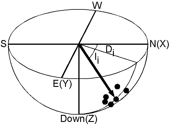
Fisher statistics is a very difficult theory, but its application to paleomagnetism is straightforward. Using declination \(D\) and inclination \(I\), each direction is specified by a unit vector as shown in the figure. The best estimate of the true direction is given by a vector sum \({\bf R}\) of \(N\) observations (resultant vector), \begin{equation} {\bf R} = (\sum_{i=1}^N \cos D_i \cos I_i, \sum_{i=1}^N \sin D_i \cos I_i, \sum_{i=1}^N \sin I_i). \label{eq02} \end{equation} Hence the mean direction \((D_m, I_m)\) is given by, \begin{equation} \tan D_m = \frac{R_Y}{R_X}, \quad \sin I_m = \frac{R_Z}{R}. \label{eq03} \end{equation} The best estimate \(k\) of \(\kappa\), for \(\kappa\) > 3, is given by, \begin{equation} k = \frac{N - 1}{N - R}. \label{eq04} \end{equation} Fisher (1953) further proved that \({\bf R}\) is also Fisher distributed with precision \(\kappa R\) and the confidence angle of the true direction with probability \((1 - P)\) is given by, \begin{equation} \cos \alpha_{(1-P)} = 1 - \frac{N-R}{R}\left[\left(\frac{1}{P}\right)^{\frac{1}{N-1}} - 1\right]. \label{eq05} \end{equation} We normally take \(P=0.05\) and \eqref{eq05} gives \(95\%\) confidence circle \(\alpha_{95}\) around the mean direction.
Angular standard deviation \(S\), or angular dispersion, is defined as, \begin{equation} S^2 = \frac{1}{N-1} \sum_{i=1}^N \theta_i^2. \label{eq06} \end{equation} Using the relation, \(\cos\theta \approx 1 - \frac{\theta^2}{2}\) for \(\theta \ll 1\), \eqref{eq06} is approximated as, \begin{eqnarray*} S^2 & \approx & \frac{1}{N-1}\sum_{i=1}^N(2 - 2\cos\theta_i) \\ & = & \frac{1}{N-1}(2\sum_{i=1}^N 1 - 2 \sum_{i=1}^N \cos\theta_i) = 2\frac{N-R}{N-1} = \frac{2}{k}. \end{eqnarray*} Hence, for a large \(k\), \begin{equation} S \approx \frac{81}{\sqrt{k}} \quad \mathsf{[deg.]}. \label{eq07} \end{equation}
This angle is often written as \(\theta_{63}\). This is originated from the case of 2-dimensional normal distribution in which 63% of observations lie within one standard deviation while the percentage is 68% in 1-D case. This is shown by considering the probability density of 2-D normal distribution, \[ {\scriptsize \frac{1}{\sqrt{2\pi}\sigma}}e^{-x^2/2\sigma^2}{\scriptsize \frac{1}{\sqrt{2\pi}\sigma}}e^{-y^2/2\sigma^2}dxdy = {\scriptsize \frac{1}{2\pi\sigma^2}}e^{-r^2/2\sigma^2}rdrd\varphi, \] where \(x=r\cos\varphi\) and \(y=r\sin\varphi\). As the variance of \(r\) is \(\sigma^2+\sigma^2=2\sigma^2\), integrating the probability density, \[ \frac{1}{\sigma^2}\int_0^{\sqrt{2}\sigma}re^{-r^2/2\sigma^2}dr = \left[-e^{-r^2/2\sigma^2}\right]_0^{\sqrt{2}\sigma} = 1 - e^{-1} = 0.6321. \] Applying this idea to the case of Fisher distribution and using \eqref{eq01}, \[ \frac{\kappa}{2\sinh\kappa}\int_0^{\theta_{63}}e^{\kappa\cos\theta}\sin\theta d\theta = \frac{e^\kappa-e^{\kappa\cos\theta_{63}}}{e^\kappa-e^{-\kappa}} = 0.6321. \] Solving this equation for \(\cos\theta_{63}\), \[ \cos\theta_{63} = 1 + \frac{\log\left(1 - 0.6321(1 - e^{-2\kappa})\right)}{\kappa} \] Using approximation for \(\kappa \gg 1\) and \(\theta_{63} \ll 1\), \begin{eqnarray*} 1 - \frac{\theta_{63}^2}{2} & \approx & 1 + \frac{\log 0.3679}{\kappa}, \\ \theta_{63}^2 & \approx & \frac{2}{\kappa}. \end{eqnarray*} Approximating \(\kappa\) by \(k\), this becomes the same expression as the angular standard deviation \(S\) given by \eqref{eq07}.
Approximated expression is also useful for a small \(\alpha_{95}\). \eqref{eq05} is approximated as the followings. \[ 1 - \frac{\alpha_{95}^2}{2} = 1 - \frac{N-R}{R}\left(20^\frac{1}{N-1} - 1\right). \] Using the relation, \(\log(1+x) \approx x\) for \(x \ll 1\), \[ \log 20^\frac{1}{N-1} = \log\left[1 + \left(20^\frac{1}{N-1} -1\right)\right] \approx 20^\frac{1}{N-1} - 1. \] Using this relation, \[ \alpha_{95}^2 \approx \frac{2(N-R)}{R} \log 20^\frac{1}{N-1} = \frac{2(N-R)}{R(N-1)} \log 20. \] Hence, \[ \alpha_{95}^2 \approx \frac{2\log 20}{kR}. \] Lastly, \(R\) is approximated by \(N\), \begin{equation} \alpha_{95} \approx \frac{140}{\sqrt{kN}} \quad \mathsf{[deg.]}. \label{eq08} \end{equation}
Reference:
- Fisher, R. A., Dispersion on a sphere, Proc. Roy. Soc., A 217, 295-305, 1953.