Bingham distribution
Paleodirections we observe are sometimes in elongated distribution although we usually analyze them with Fisher statistics supposing that they are circularly symmetric. One of the statistics to describe elongated distribution on the unit sphere was given by Bingham (1974). The Bingham statistics is a very difficult theory but its application to paleomagnetism is easy if numerical procedure is adopted (Onstott, 1980). Concise introduction to the method is contained in Tanaka (1999).
Suppose we have \(N\) paleodirections with some dispersion, each of which is designated by a unit vector \({\bf L}_i=(x_i,y_i,z_i)\). We first analyze the distribution of the data points by the following orientation matrix: \begin{equation} {\bf T} = \left(\begin{array}{ccc} \sum_{i=1}^N x_i^2 & \sum_{i=1}^N x_i y_i & \sum_{i=1}^N x_i z_i \\ \sum_{i=1}^N x_i y_i & \sum_{i=1}^N y_i^2 & \sum_{i=1}^N y_i z_i \\ \sum_{i=1}^N x_i z_i & \sum_{i=1}^N y_i z_i & \sum_{i=1}^N z_i^2 \end{array}\right). \label{eq01} \end{equation} Similar to the principal component analysis, eigenvalues of \({\bf T}\), \(\tau_1\), \(\tau_2\), and \(\tau_3\) (\(\tau_1 \leq \tau_2 \leq \tau_3\), \(\tau_1 + \tau_2 + \tau_3 = N\)) and corresponding eigenvectors \({\bf t}_1\), \({\bf t}_2\), and \({\bf t}_3\), collectively give the structure of the data points distribution. In the typical case of paleodirections with moderate dispersion (\(\tau_1 \leq \tau_2 \ll \tau_3\)), \({\bf t}_3\) gives the mean direction and the larger difference of \(\tau_2\) and \(\tau_1\) indicates the larger elongation along \({\bf t}_2\) direction. In the case of girdle-like coplanar distribution (\(\tau_1 \ll \tau_2 \leq \tau_3\)), \({\bf t}_1\) indicates a pole to the plane of the girdle.
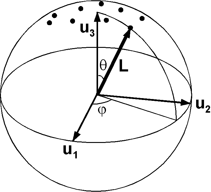
The probability density of the Bingham distribution is given by \[ b = \frac{1}{4\pi d(k_1,k_2,k_3)} e^{k_1({\bf L}\cdot{\bf u}_1)^2} e^{k_2({\bf L}\cdot{\bf u}_2)^2} e^{k_3({\bf L}\cdot{\bf u}_3)^2}, \] where \({\bf u}_1\), \({\bf u}_2\), and \({\bf u}_3\) are the true eigenvectors, \(k_1\), \(k_2\), and \(k_3\) are concentration parameters, and \(d(k_1,k_2,k_3)\) is a normalization factor. It was shown that \(\tau_1\), \(\tau_2\), and \(\tau_3\) and \({\bf t}_1\), \({\bf t}_2\), and \({\bf t}_3\) are the best estimates of the true eigenvalues and eigenvectors, respectively. It was also shown that \(k_3\) can be set to zero without losing generality. Taking the coordinates, \(\theta\) and \(\varphi\), as shown in the figure, the Bingham density function is reduced to \begin{equation} b(\theta,\varphi) = \frac{1}{4\pi d(k_1,k_2)} e^{(k_1\cos^2\varphi + k_2\sin^2\varphi)\sin^2\theta}, \label{eq02} \end{equation} where the normalization constant \(d(k_1,k_2)\) is given by \begin{equation} d(k_1,k_2) = \frac{1}{4\pi} \int_0^{2\pi}\int_0^\pi e^{(k_1\cos^2\varphi + k_2\sin^2\varphi)\sin^2\theta} \sin\theta d\theta d\varphi. \label{eq03} \end{equation} As analytical solution of \eqref{eq03} is unavailable, \(d(k_1,k_2)\) is determined numerically.
The maximum likelihood estimates of \(k_1\) and \(k_2\) are determined by maximizing the log-likelihood function for the Bingham distribution: \begin{eqnarray*} F & = & \log \prod_{i=1}^N \frac{1}{4\pi d(k_1,k_2)} e^{(k_1\cos^2\varphi_i + k_2\sin^2\varphi_i)\sin^2\theta_i} \\ & = & -N\log 4\pi - N\log d(k_1,k_2) + k_1\sum_{i=1}^N \cos^2\varphi_i\sin^2\theta_i + k_2\sum_{i=1}^N \sin^2\varphi_i\sin^2\theta_i. \end{eqnarray*} Concerning to the last two terms, \(\cos\varphi_i\sin\theta_i\) and \(\sin\varphi_i\sin\theta_i\) are the component of \({\bf L}_i\) along the eigenvectors \({\bf u}_1\) and \({\bf u}_2\), respectively. Because sum of the squares of the component along the eigenvector equals to the corresponding eigenvalue, the log-likelihood function becomes \begin{equation} F = -N\log 4\pi - N\log d(k_1,k_2) + k_1\tau_1 + k_2\tau_2. \label{eq04} \end{equation} Finding \(k_1\) and \(k_2\) which maximize \eqref{eq04} on the condition \eqref{eq03} is not difficult by using a maximization routine. Bingham (1974) also showed that 95\(\%\) confidence radii around the eigenvector \({\bf t}_3\) are given by \begin{equation} \alpha_{31} = 2.45\sigma_{31}, \quad \alpha_{32} = 2.45\sigma_{32}, \label{eq05} \end{equation} where \(\alpha_{31}\) and \(\alpha_{32}\) indicate radii along \({\bf t}_1\) and \({\bf t}_2\) directions, respectively, and \(\sigma_{ij}\) is given by \begin{equation} \sigma_{ij}^2 = \frac{1}{2(k_i - k_j)(\tau_i - \tau_j)}. \label{eq06} \end{equation}
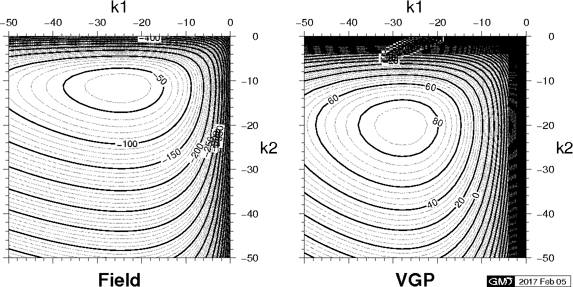
Bingham statistics was applied to 324 paleodirections observed at Hawaii Island for the last 5 Myr (→figure). Owing to \(\sin^2\theta\) dependence of the Bingham distribution, both polarities were analyzed at the same time. The results are summarized in the table which indicates that elongation along meridian is observed in field directions while the distribution of VGPs is almost circular. Last figures are contour maps of \(F\) against \(k_1\) and \(k_2\) in the analysis of the Hawaii data, which are free of any local maxima.
| \(k_1\) | \(k_2\) | \(\tau_1\) | \(\tau_2\) | \(\alpha_{31}\) | \(\alpha_{32}\) | |
| Field | -24.6 | -11.3 | 6.74 | 15.12 | 1.16° | 1.74° |
| VGP | -27.8 | -20.0 | 5.95 | 8.34 | 1.08° | 1.28° |
Contour map of \(F\) against \(k_1\) and \(k_2\) in the analysis of Bingham statistics.
Reference:
- Bingham, C., An antipodally symmetric distribution on the sphere, Ann. Statistics, 2, 1201-1225, 1974.
- Onstott, T. C., Application of the Bingham distribution function in paleomagnetic studies, J. Geophys. Res., 85, 1500-1510, 1980.
- Tanaka, H., Circular asymmetry of the paleomagnetic directions observed at low latitude volcanic sites, Earth Planets Space, 51, 1279-1286, 1999. (→doi:10.1186/BF03351601)