Line fitting of y = a + bx: Special solution of York (1966)
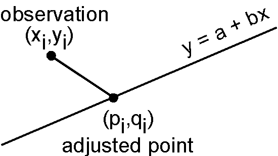 For analyzing an Arai plot in paleointensity experiments, Coe et al. (1978) proposed to use a special solution of York (1966). In York's theory the quantity to be minimized is given by,
\[ t = \sum_{i=1}^n \{w(x_i)(x_i - p_i)^2 + w(y_i)(y_i - q_i)^2\}, \]
where \(w(x_i)\) and \(w(y_i)\) are the weights of the observations. The theory develops very complicated general equations for \(b\) which are not described here. Among easier special solutions, when
\[ \frac{w(x_i)}{w(y_i)} = c \quad (\mathsf{constant}) \]
the equation is given by,
\[
\left( \sum_{i=1}^n w(x_i) u_i v_i \right)b^2
- \left( \sum_{i=1}^n w(x_i) v_i^2 - c\sum_{i=1}^n w(x_i) u_i^2 \right)b
- c\sum_{i=1}^n w(x_i) u_i v_i = 0,
\]
where
\[ u_i = x_i - \bar x, \quad v_i = y_i - \bar y. \]
There are three cases for this special equation, and Coe et al. (1978) proposed to use the last case;
\[
w(x_i) = \frac{1}{\sigma_x^2} = \frac{n-1}{\sum_{i=1}^n u_i^2}, \quad
w(y_i) = \frac{1}{\sigma_y^2} = \frac{n-1}{\sum_{i=1}^n v_i^2}.
\]
Then \(b\) is given by the following simple equation,
\begin{equation}
b = \sqrt{ \frac{\sum_{i=1}^n v_i^2}{\sum_{i=1}^n u_i^2} } = \frac{\sigma_y}{\sigma_x}. \label{eq01}
\end{equation}
York (1966) also gave an estimate of \(\sigma_b\) as,
\begin{equation}
\sigma_b^2 = \frac{1}{n-2}\frac{2\sum_{i=1}^n v_i^2 - 2b\sum_{i=1}^n u_i v_i}{\sum_{i=1}^n u_i^2}, \label{eq02}
\end{equation}
which is called a standard error of \(b\).
For analyzing an Arai plot in paleointensity experiments, Coe et al. (1978) proposed to use a special solution of York (1966). In York's theory the quantity to be minimized is given by,
\[ t = \sum_{i=1}^n \{w(x_i)(x_i - p_i)^2 + w(y_i)(y_i - q_i)^2\}, \]
where \(w(x_i)\) and \(w(y_i)\) are the weights of the observations. The theory develops very complicated general equations for \(b\) which are not described here. Among easier special solutions, when
\[ \frac{w(x_i)}{w(y_i)} = c \quad (\mathsf{constant}) \]
the equation is given by,
\[
\left( \sum_{i=1}^n w(x_i) u_i v_i \right)b^2
- \left( \sum_{i=1}^n w(x_i) v_i^2 - c\sum_{i=1}^n w(x_i) u_i^2 \right)b
- c\sum_{i=1}^n w(x_i) u_i v_i = 0,
\]
where
\[ u_i = x_i - \bar x, \quad v_i = y_i - \bar y. \]
There are three cases for this special equation, and Coe et al. (1978) proposed to use the last case;
\[
w(x_i) = \frac{1}{\sigma_x^2} = \frac{n-1}{\sum_{i=1}^n u_i^2}, \quad
w(y_i) = \frac{1}{\sigma_y^2} = \frac{n-1}{\sum_{i=1}^n v_i^2}.
\]
Then \(b\) is given by the following simple equation,
\begin{equation}
b = \sqrt{ \frac{\sum_{i=1}^n v_i^2}{\sum_{i=1}^n u_i^2} } = \frac{\sigma_y}{\sigma_x}. \label{eq01}
\end{equation}
York (1966) also gave an estimate of \(\sigma_b\) as,
\begin{equation}
\sigma_b^2 = \frac{1}{n-2}\frac{2\sum_{i=1}^n v_i^2 - 2b\sum_{i=1}^n u_i v_i}{\sum_{i=1}^n u_i^2}, \label{eq02}
\end{equation}
which is called a standard error of \(b\).
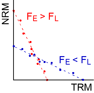
The above \(\sigma_x^2\) and \(\sigma_y^2\) used for the weights \(w(x_i)\) and \(w(y_i)\) do not necessarily reflect the errors of \(x_i\) and \(y_i\) because they are variances around the means. Nevertheless, they conform with the general idea of the errors in the Arai plot; the absolute value of measurements error is proportional to the remanence intensity. In this case, as known from the figure, the errors of \(x_i\) and \(y_i\) can be expressed as, \[ \sigma_{x_i}^2 = (F_L \sigma)^2, \quad \sigma_{y_i}^2 = (F_E \sigma)^2, \] where \(F_L\) and \(F_E\) are strength of the laboratory and paleo fields, respectively, and \(\sigma\) is a constant which reflects a general error of the measurements. Hence, the above \(b\) and \(\sigma_b\) given by \eqref{eq01} and \eqref{eq02} are considered to be reasonable.
References:
- Coe, R. S., S. Gromme, and E. A. Mankinen, Geomagnetic paleointensities from radiocarbon-dated lava flows on Hawaii and the question of the Pacific nondipole low,J. Geophys. Res., 83, 1740-1756, 1978.
- York, D., Least-squares fitting of a straight line,Can. J. Phys., 44, 1079-1086, 1966.