Principal component analysis
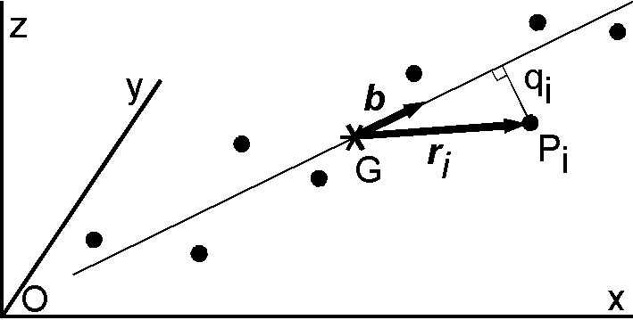 The principal component analysis (PCA) is useful to analyze paleomagnetic data (Kirschvink, 1980). Application of PCA to determine a remanence direction is illustrated in the figure in which each data point indicates the end point of remanence during demagnetization procedure. The remanence direction is an axis which minimizes the total moment of inertia, \(I\), of the data points. Supposing a unit mass for each data point \(P_i\), \(I\) is given by,
\begin{eqnarray*}
I & = & \sum_{i=1}^N 1 \times q_i^2 \\
& = & \sum_{i=1}^N \{|{\bf r}_i|^2 - ({\bf b}\cdot{\bf r}_i)^2\}
= \sum_{i=1}^N |{\bf r}_i|^2 - \sum_{i=1}^N ({\bf b}\cdot{\bf r}_i)^2
\end{eqnarray*}
where \(q_i\) is the distance of \(P_i\) from the axis, \({\bf r}_i\) is a vector pointing to \(P_i\) from the center of gravity \(G\), and \({\bf b}\) is a unit vector along the axis. To seek \({\bf b}\) which minimize \(I\) is equivalent to seek \({\bf b}\) which maximize the second term. To conform with the conventional PCA, we maximize \(\frac{1}{N}\sum_{i=1}^N({\bf b}\cdot{\bf r}_i)^2\) on the condition \(|{\bf b}|=1\). Using Lagrange's multiplier \(\lambda\), we maximize
\[
{\cal F} = \frac{1}{N}\sum_{i=1}^N({\bf b}\cdot{\bf r}_i)^2 - \lambda({\bf b}\cdot{\bf b}-1)
\]
Introducing a matrix \({\bf A}\),
\[
{\bf A} = \left(\begin{array}{lll}
\frac{1}{N}\sum_{i=1}^N(x_i-\bar x)^2 & \frac{1}{N}\sum_{i=1}^N(x_i-\bar x)(y_i-\bar y) &
\frac{1}{N}\sum_{i=1}^N(x_i-\bar x)(z_i-\bar z) \\
\frac{1}{N}\sum_{i=1}^N(x_i-\bar x)(y_i-\bar y) & \frac{1}{N}\sum_{i=1}^N(y_i-\bar y)^2 &
\frac{1}{N}\sum_{i=1}^N(y_i-\bar y)(z_i-\bar z) \\
\frac{1}{N}\sum_{i=1}^N(x_i-\bar x)(z_i-\bar z) &
\frac{1}{N}\sum_{i=1}^N(y_i-\bar y)(z_i-\bar z) & \frac{1}{N}\sum_{i=1}^N(z_i-\bar z)^2
\end{array}\right)
\]
where \({\bf r}_i = (x_i-\bar x,y_i-\bar y,z_i-\bar z)\), \({\cal F}\) is given as,
\[
{\cal F} = {^t{\bf b}} {\bf A} {\bf b} - \lambda(^t{\bf b}{\bf b} - 1).
\]
Setting \(\partial{\cal F}/\partial{\bf b}=2{\bf A}{\bf b}-2\lambda{\bf b}=0\), we obtain,
\begin{equation}
{\bf A}{\bf b} = \lambda{\bf b}. \label{eq01}
\end{equation}
The principal component analysis (PCA) is useful to analyze paleomagnetic data (Kirschvink, 1980). Application of PCA to determine a remanence direction is illustrated in the figure in which each data point indicates the end point of remanence during demagnetization procedure. The remanence direction is an axis which minimizes the total moment of inertia, \(I\), of the data points. Supposing a unit mass for each data point \(P_i\), \(I\) is given by,
\begin{eqnarray*}
I & = & \sum_{i=1}^N 1 \times q_i^2 \\
& = & \sum_{i=1}^N \{|{\bf r}_i|^2 - ({\bf b}\cdot{\bf r}_i)^2\}
= \sum_{i=1}^N |{\bf r}_i|^2 - \sum_{i=1}^N ({\bf b}\cdot{\bf r}_i)^2
\end{eqnarray*}
where \(q_i\) is the distance of \(P_i\) from the axis, \({\bf r}_i\) is a vector pointing to \(P_i\) from the center of gravity \(G\), and \({\bf b}\) is a unit vector along the axis. To seek \({\bf b}\) which minimize \(I\) is equivalent to seek \({\bf b}\) which maximize the second term. To conform with the conventional PCA, we maximize \(\frac{1}{N}\sum_{i=1}^N({\bf b}\cdot{\bf r}_i)^2\) on the condition \(|{\bf b}|=1\). Using Lagrange's multiplier \(\lambda\), we maximize
\[
{\cal F} = \frac{1}{N}\sum_{i=1}^N({\bf b}\cdot{\bf r}_i)^2 - \lambda({\bf b}\cdot{\bf b}-1)
\]
Introducing a matrix \({\bf A}\),
\[
{\bf A} = \left(\begin{array}{lll}
\frac{1}{N}\sum_{i=1}^N(x_i-\bar x)^2 & \frac{1}{N}\sum_{i=1}^N(x_i-\bar x)(y_i-\bar y) &
\frac{1}{N}\sum_{i=1}^N(x_i-\bar x)(z_i-\bar z) \\
\frac{1}{N}\sum_{i=1}^N(x_i-\bar x)(y_i-\bar y) & \frac{1}{N}\sum_{i=1}^N(y_i-\bar y)^2 &
\frac{1}{N}\sum_{i=1}^N(y_i-\bar y)(z_i-\bar z) \\
\frac{1}{N}\sum_{i=1}^N(x_i-\bar x)(z_i-\bar z) &
\frac{1}{N}\sum_{i=1}^N(y_i-\bar y)(z_i-\bar z) & \frac{1}{N}\sum_{i=1}^N(z_i-\bar z)^2
\end{array}\right)
\]
where \({\bf r}_i = (x_i-\bar x,y_i-\bar y,z_i-\bar z)\), \({\cal F}\) is given as,
\[
{\cal F} = {^t{\bf b}} {\bf A} {\bf b} - \lambda(^t{\bf b}{\bf b} - 1).
\]
Setting \(\partial{\cal F}/\partial{\bf b}=2{\bf A}{\bf b}-2\lambda{\bf b}=0\), we obtain,
\begin{equation}
{\bf A}{\bf b} = \lambda{\bf b}. \label{eq01}
\end{equation}
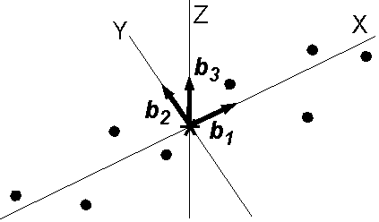
Solving equation \eqref{eq01} which is an eigenvalue problem, three eigenvalues \((\lambda_1 \geq \lambda_2 \geq \lambda_3)\) and corresponding eigenvectors \(({\bf b}_1,{\bf b}_2,{\bf b}_3)\) give a general idea of the distribution of the data points. In the case of a linear remanence as shown in the figure \((\lambda_1 \gg \lambda_2 \geq \lambda_3)\), \({\bf b}_1\) gives the best fitted remanence direction while \(\lambda_1\) is the variance along the \({\bf b}_1\) direction (\(\sigma_1^2\)). In fact, taking \(X\) axis along \({\bf b}_1\) with an origin \(O\) at \(G\), the variance of \(X\) is given as, \begin{eqnarray*} \sigma_1^2 & = & \frac{1}{N}\sum_{i=1}^N X_i^2 = \frac{1}{N}\sum_{i=1}^N ({\bf b}_1\cdot{\bf r}_i)^2 \\ & = & {^t{\bf b}}_1{\bf A}{\bf b}_1 = {^t{\bf b}}_1(\lambda_1{\bf b}_1) = \lambda_1(^t{\bf b}_1{\bf b}_1) = \lambda_1. \end{eqnarray*} Taking \(Y\) and \(Z\) axes along \({\bf b}_2\) and \({\bf b}_3\), respectively, the covariance of different axes becomes zero. In fact, the covariance of \(X\) and \(Y\) (\(\gamma_{12}\)) is given as, \begin{eqnarray*} \gamma_{12} & = & \frac{1}{N}\sum_{i=1}^N X_i Y_i = \frac{1}{N}\sum_{i=1}^N ({\bf b}_1\cdot{\bf r}_i)({\bf b}_2\cdot{\bf r}_i) \\ & = & {^t{\bf b}}_1{\bf A}{\bf b}_2 = {^t{\bf b}}_1(\lambda_2{\bf b}_2) = \lambda_2(^t{\bf b}_1{\bf b}_2) = 0. \end{eqnarray*} As each eigenvalue is the square of the standard deviation (\(\sigma^2\)) along each axis of eigenvector, Kirschvink (1980) proposed to use them to represent the error of the best fitted line. For this purpose Maximum Angular Deviation (MAD) was introduced as, \begin{equation} MAD = \arctan\left(\frac{\sqrt{\sigma_2^2+\sigma_3^2}}{\sigma_1}\right) = \arctan\left(\sqrt{\frac{\lambda_2+\lambda_3}{\lambda_1}}\right). \label{eq02} \end{equation}
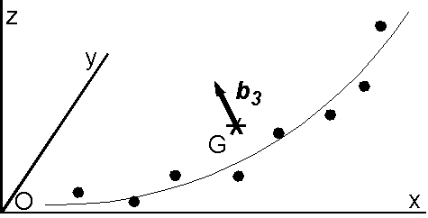
When the remanence contains two components it often happens that the end point of the remanence vector follows a circle-like coplanar path during demagnetization procedure as shown in the figure. In such a case one eigenvalue is much smaller than the other two (\(\lambda_3 \ll \lambda_2 \leq \lambda_1\)) and the eigenvector \({\bf b}_3\) corresponding to \(\lambda_3\) indicates a pole to the plane. Kirschvink (1980) suggested the next MAD as an error of the pole. \begin{equation} MAD = \arctan\left(\sqrt{\frac{\sigma_3^2}{\sigma_2^2}+\frac{\sigma_3^2}{\sigma_1^2}}\right) = \arctan\left(\sqrt{\frac{\lambda_3}{\lambda_2}+\frac{\lambda_3}{\lambda_1}}\right). \label{eq03} \end{equation}
Reference:
- Kirschvink, J. L., The least-squares line and plane and the analysis of paleomagnetic data, Geophys. J. R. astr. Soc., 62, 699-718, 1980.