Eccentric dipole: Gauss coefficients and dipole offset
Supposing that there is no electric current on the earth's surface, geomagnetic field (magnetic induction) is given by gradient of a scalar potential \(W\), \[ {\bf B} = -\nabla W. \] As \(\nabla\cdot{\bf B}=0\), potential \(W\) satisfies Laplace's equation; \[ \nabla^2 W = 0. \] Solving this equation in spherical coordinates, \(W\) for the field of internal origin is represented by spherical harmonics as, \begin{equation} W = a\sum_{n=1}^\infty\sum_{m=0}^n\left(\frac{a}{r}\right)^{n+1}P_n^m(\cos\theta)(g_n^m\cos m\phi + h_n^m\sin m\phi), \label{eq01} \end{equation} where \(a\) is the radius of the earth, \((r,\theta,\phi)\) is an observation point (\(r\geq a\)), and \(P_n^m(\cos\theta)\) is quasi-normalized Schmidt function (associated Legendre polynomials). \(g_n^m\) and \(h_n^m\) are called Gauss coefficients and have the unit of magnetic induction (T). In 1830's, Carl Friedrich Gauss first determined the Gauss coefficients by the least squares method, and showed that the geomagnetic field is mostly internal origin and similar to a geocentric dipole field. Since 1900, the Gauss coefficients have been reported for every five years as International Geomagnetic Reference Field (IGRF). Those for 2020 of IGRF-13 (IAGA Working Group V-MOD, 2020) are shown from \(n\)=1 to 3 in the unit of nT (10\(^{-9}\)T) in the next table.
| \(n\) | \(m\) | \(g\) | \(h\) | \(n\) | \(m\) | \(g\) | \(h\) | \(n\) | \(m\) | \(g\) | \(h\) | ||||
| 1 | 0 | -29404.8 | 0.0 | 2 | 0 | -2499.6 | 0.0 | 3 | 0 | 1363.2 | 0.0 | ||||
| 1 | 1 | -1450.9 | 4652.5 | 2 | 1 | 2982.0 | -2991.6 | 3 | 1 | -2381.2 | -82.1 | ||||
| 2 | 2 | 1677.0 | -734.6 | 3 | 2 | 1236.2 | 241.9 | ||||||||
| 3 | 3 | 525.7 | -543.4 |
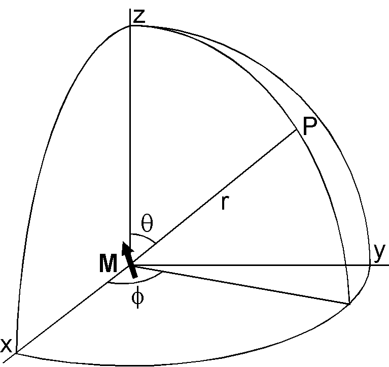
As seen from the above table, contribution of \(n\)=1 to the geomagnetic field is much larger than the higher terms. The fact that the \(n\)=1 terms indicate the geocentric dipole field is shown by the followings. Consider the magnetic potential of a geocentric dipole shown in the right figure; \begin{eqnarray*} W & = & \frac{\mu_0}{4\pi}\frac{{\bf M}\cdot{\bf r}}{r^3} \\ & = & \frac{\mu_0}{4\pi r^2}\left(M_x\sin\theta\cos\phi + M_y\sin\theta\sin\phi + M_z\cos\theta\right). \end{eqnarray*} Considering \(P_1^0(\cos\theta)\)=\(\cos\theta\) and \(P_1^1(\cos\theta)\)=\(\sin\theta\), equation \eqref{eq01} for \(n\)=1 is given by, \[ W = \frac{a^3}{r^2}(g_1^0 \cos\theta + g_1^1 \sin\theta \cos\phi + h_1^1 \sin\theta \sin\phi). \] Comparing these two expressions of the potential, we obtain the next relation of the \(n\)=1 terms and the geocentric dipole. \begin{equation} g_1^0 = \frac{\mu_0}{4\pi a^3}M_z, \quad g_1^1 = \frac{\mu_0}{4\pi a^3}M_x, \quad h_1^1 = \frac{\mu_0}{4\pi a^3}M_y. \label{eq02} \end{equation} Hence, geomagnetic field is expressed by an inclined geocentric dipole combined with higher nondipole terms, although this is simply a mathematical convenience. It would be intuitive if the nondipole terms are expressed by displacing the dipole from the center of the earth, which is called an eccentric dipole, or offset dipole.
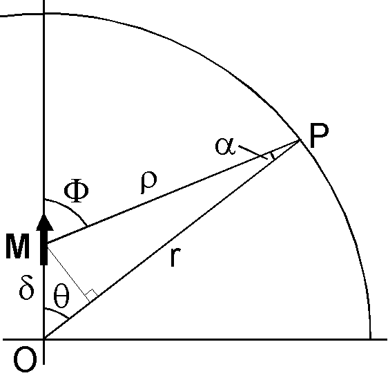
The following easy introduction to the eccentric dipole is after Lowrie (2011). First we consider the case of axial dipole displaced along the earth's rotation axis by small distance \(\delta\) (right figure). The potential of the dipole at the observation point P is given by, \begin{equation} W = \frac{\mu_0}{4\pi}\frac{M\cos\Phi}{\rho^2}. \label{eq03} \end{equation} Here \(\Phi\) and \(\rho\) are related to \(\theta\) and \(r\) by, \begin{align*} \cos\Phi & = \cos(\theta+\alpha) = \cos\theta\cos\alpha - \sin\theta\sin\alpha, \\ \rho^2 & = r^2 + \delta^2 -2r\delta\cos\theta. \end{align*} As \(\delta\) and \(\alpha\) are small, the following approximation holds. \[ \sin\alpha = \frac{\delta\sin\theta}{\rho} \approx \frac{\delta\sin\theta}{r}, \quad \cos\alpha \approx 1. \] Using these approximations, \[ \cos\Phi \approx \cos\theta - \frac{\delta}{r}\sin^2\theta, \qquad \rho^2 \approx r^2\left(1 - \frac{2\delta}{r}\cos\theta\right). \] Substituting these expressions to \eqref{eq03}, \begin{eqnarray*} W & \approx & \frac{\mu_0}{4\pi}M\left(\cos\theta - \frac{\delta}{r}\sin^2\theta\right)\left/\left(r^2\left(1 - \frac{2\delta}{r}\cos\theta\right)\right)\right., \\ & \approx & \frac{\mu_0 M}{4\pi r^2}\left(\cos\theta - \frac{\delta}{r}\sin^2\theta\right)\left(1 + \frac{2\delta}{r}\cos\theta\right), \\ & \approx & \frac{\mu_0 M}{4\pi r^2}\left(\cos\theta - \frac{\delta}{r}\sin^2\theta + \frac{2\delta}{r}\cos^2\theta\right), \\ & \approx & \frac{\mu_0 M}{4\pi r^2}\cos\theta + \frac{\mu_0 M\delta}{4\pi r^3}(3\cos^2\theta - 1), \\ & \approx & \frac{\mu_0 M}{4\pi r^2}P_1^0(\cos\theta) + \frac{\mu_0 M\delta}{2\pi r^3}P_2^0(\cos\theta). \end{eqnarray*} Comparing the last equation with \eqref{eq01} for \(n\)=1 and 2, \begin{equation} g_1^0 = \frac{\mu_0}{4\pi a^3}M, \qquad g_2^0 = \frac{\mu_0 \delta}{2\pi a^4}M. \label{eq04} \end{equation} Hence, when an axial dipole displaces along the rotation axis by small distance, \(g_2^0\) term appears.
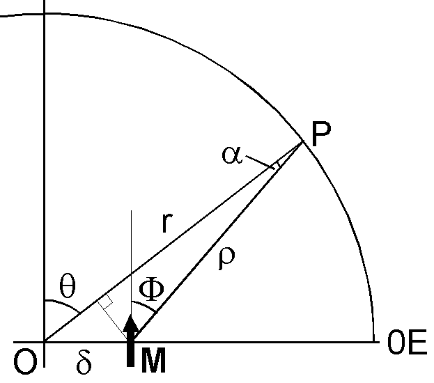
Case of a dipole displaced in the equatorial plane can be treated in a similar way. Right figure shows the geometry in which the axial dipole displaced by a small distance \(\delta\) in the equatorial plane toward the direction of 0°E. Relations of \(\Phi\), \(\theta\), \(\rho\), and \(r\) are now, \begin{align*} \cos\Phi & = \cos(\theta-\alpha) = \cos\theta\cos\alpha + \sin\theta\sin\alpha, \\ \rho^2 & = r^2 + \delta^2 -2r\delta\sin\theta. \end{align*} Approximation of \(\sin\alpha\) and \(\cos\alpha\) are, \[ \sin\alpha = \frac{\delta\cos\theta}{\rho} \approx \frac{\delta\cos\theta}{r}, \qquad \cos\alpha \approx 1. \] Hence, \[ \cos\Phi \approx \cos\theta + \frac{\delta}{r}\sin\theta\cos\theta, \qquad \rho^2 \approx r^2\left(1 - \frac{2\delta}{r}\sin\theta\right). \] The potential \eqref{eq03} is now, \begin{eqnarray*} W & \approx & \frac{\mu_0}{4\pi}M\left(\cos\theta+\frac{\delta}{r}\sin\theta\cos\theta\right)\left/\left(r^2\left(1-\frac{2\delta}{r}\sin\theta\right)\right)\right., \\ & \approx & \frac{\mu_0 M}{4\pi r^2}\left(\cos\theta+\frac{\delta}{r}\sin\theta\cos\theta\right)\left(1+\frac{2\delta}{r}\sin\theta\right), \\ & \approx & \frac{\mu_0 M}{4\pi r^2}\left(\cos\theta+\frac{3\delta}{r}\sin\theta\cos\theta\right), \\ & \approx & \frac{\mu_0 M}{4\pi r^2}P_1^0(\cos\theta) + \frac{\sqrt{3}\mu_0 M\delta}{4\pi r^3}P_2^1(\cos\theta). \end{eqnarray*} Comparing the last equation with \eqref{eq01} for \(n\)\(\leq\)2 and \(\phi\)=0, \begin{equation} g_1^0 = \frac{\mu_0}{4\pi a^3}M, \qquad g_2^1 = \frac{\sqrt{3}\mu_0 \delta}{4\pi a^4}M. \label{eq05} \end{equation} In the above figure, both the eccentric dipole and the observation point are in the Greenwich meridional plane. With more detailed derivation (next page), it will be shown that displacements in 0°E and 90°E directions cause appearance of \(g_2^1\) and \(h_2^1\) terms, respectively. It can be concluded that, in general, small displacement of the axial dipole in the equatorial plane causes appearance of \(g_2^1\) and \(h_2^1\) terms.
References:
- IAGA Working Group V-MOD, International Geomagnetic Reference Field: IGRF-13 is released, 2020. (URL: https://www.ngdc.noaa.gov/IAGA/vmod/igrf.html)
- Lowrie, W., A Student's Guide to Geophysical Equations, 281 pp., Cambridge University Press, Cambridge, 2011.