Stream function for drawing lines of magnetic field
Static magnetic field \({\bf H}\) is given by gradient of a magnetic potential \(W\), \begin{equation} {\bf H} = -\nabla W. \label{eq01} \end{equation} Considering two dimensional case, \({\bf H}\) is perpendicular to the line of equi-potential; \(W = \mathsf{const.}\) Hence, if we find a scalar function \(\phi\) which is perpendicular to \(W\), the line of \(\phi = \mathsf{const.}\) will give the field line. \(\phi\) is called a stream function, and hereafter easy introduction to its principle is given together with application to drawing field lines of a dipole moment.
As the magnetic field to be considered is static in vacuum, \[ \nabla\cdot{\bf H} = (1/\mu_0)\nabla\cdot{\bf B} = 0. \] Using this relation in two dimensional orthogonal coordinate system, \[ \nabla\cdot{\bf H} = \frac{\partial H_x}{\partial x} + \frac{\partial H_y}{\partial y} = 0. \] Substituting \eqref{eq01}, i.e., \(H_x=-\partial W/\partial x\) and \(H_y=-\partial W/\partial y\), \begin{equation} \frac{\partial}{\partial x}\left(\frac{\partial W}{\partial x}\right) = -\frac{\partial}{\partial y}\left(\frac{\partial W}{\partial y}\right). \label{eq02} \end{equation} Here, we introduce another scalar function \(\phi\) as, \[ \frac{\partial W}{\partial x} = \frac{\partial \phi}{\partial y}, \qquad \frac{\partial W}{\partial y} = -\frac{\partial \phi}{\partial x}. \] The new scalar function \(\phi\) satisfies \eqref{eq02} and is perpendicular to the potential \(W\) because \(\nabla\phi\cdot\nabla W=0\). \({\bf H}\) is also expressed by \(\phi\); \(H_x=-\partial\phi/\partial y\) and \(H_y=\partial\phi/\partial x\).
Next we consider a case in two dimensional polar coordinate system. \[ \nabla\cdot{\bf H} = \frac{1}{r^2}\frac{\partial}{\partial r}\left(r^2H_r\right) + \frac{1}{r\sin\theta}\frac{\partial}{\partial\theta}\left(\sin\theta H_\theta\right) = 0. \] Hence, \[ \frac{1}{r^2}\frac{\partial}{\partial r}\left(r^2H_r\right) = -\frac{1}{r\sin\theta}\frac{\partial}{\partial\theta}\left(\sin\theta H_\theta\right). \] Substituting \eqref{eq01}, i.e., \(H_r=-\partial W/\partial r\) and \(H_\theta=-(1/r)\partial W/\partial\theta\), the next equation is obtained. \begin{equation} \frac{\partial}{\partial r}\left(r^2\frac{\partial W}{\partial r}\right) = -\frac{1}{\sin\theta}\frac{\partial}{\partial\theta}\left(\sin\theta\frac{\partial W}{\partial\theta}\right). \label{eq03} \end{equation} By examining \eqref{eq03}, we find that the stream function \(\phi\) should satisfy the next relation; \begin{equation} r^2\frac{\partial W}{\partial r} = \frac{1}{\sin\theta}\frac{\partial\phi}{\partial\theta}, \qquad \sin\theta\frac{\partial W}{\partial\theta} = -\frac{\partial\phi}{\partial r}. \label{eq04} \end{equation} Orthogonality of \(\phi\) and \(W\) is ascertained as, \begin{eqnarray*} \nabla\phi\cdot\nabla W & = & \frac{\partial\phi}{\partial r}\frac{\partial W}{\partial r} + \frac{1}{r}\frac{\partial\phi}{\partial\theta}\frac{1}{r}\frac{\partial W}{\partial\theta} \\ & = & \frac{1}{r^2\sin\theta}\frac{\partial\phi}{\partial r}\frac{\partial\phi}{\partial\theta} - \frac{1}{r^2\sin\theta}\frac{\partial\phi}{\partial\theta}\frac{\partial\phi}{\partial r} = 0. \end{eqnarray*} \({\bf H}\) is also given by \(\phi\) as, \begin{equation} H_r = -\frac{\partial W}{\partial r} = -\frac{1}{r^2\sin\theta}\frac{\partial\phi}{\partial\theta}, \qquad H_\theta = -\frac{1}{r}\frac{\partial W}{\partial\theta} = \frac{1}{r\sin\theta}\frac{\partial\phi}{\partial r}. \label{eq05} \end{equation}
Above results are now applied to the case of a magnetic dipole moment which is placed at the origin of two dimensional polar coordinate system. The potential \(W\) of the magnetic dipole moment \({\bf m}\) which points to the direction of \(\theta=0\) is given by, \begin{equation} W = \frac{m}{4\pi}\frac{\cos\theta}{r^2}. \label{eq06} \end{equation} Substituting \eqref{eq06} to equation \eqref{eq04} which \(\phi\) should satisfy, we find that \(\phi\) is given by, \begin{equation} \phi = -\frac{m}{4\pi}\frac{\sin^2\theta}{r}. \label{eq07} \end{equation} Orthogonality of the obtained \(\phi\) and \(W\) is easily ascertained by calculating \(\nabla\phi\cdot\nabla W\) which is zero. Substituting \eqref{eq07} to \eqref{eq05}, \(H_r\) and \(H_\theta\) are given by, \begin{equation} H_r = -\frac{1}{r^2\sin\theta}\frac{\partial\phi}{\partial\theta} = \frac{m}{2\pi}\frac{\cos\theta}{r^3}, \qquad H_\theta = \frac{1}{r\sin\theta}\frac{\partial\phi}{\partial r} = \frac{m}{4\pi}\frac{\sin\theta}{r^3}. \label{eq08} \end{equation} which are the same as those derived from the potential \(W\).
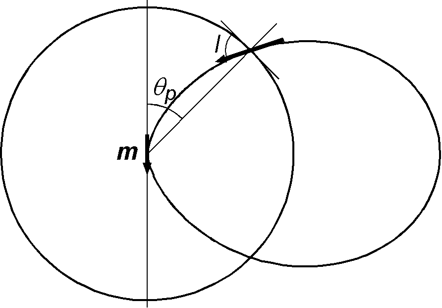
Using \eqref{eq07}, it is easy to draw lines of dipole field by plotting \(r\) versus \(\theta\) while setting \(\phi\) constant. Nevertheless, they should be drawn by taking the flux density \({\bf B}\) into consideration. As shown in the figure, we consider a flux density function \(f(\theta_p)\) at the point of colatitude \(\theta_p\) on a sphere of unit radius (\(m\) is negative simulating earth's magnetic field). As the flux density is proportional to \(|{\bf H}|\) in vacuum, using \eqref{eq08} with \(r=1\), \[ f(\theta_p) \propto \sqrt{1 + 3\cos^2\theta_p}. \] Considering the inclined magnetic field on the surface of the sphere, the flux density is multiplied by \(\sin I\) where \(I\) is an angle (inclination) between the field line and the tangent of the sphere. Hence, \[ f(\theta_p) \propto \sin I \sqrt{1 + 3\cos^2\theta_p}. \] Using that \(I\) is related to \(\theta_p\) by \(\tan I = 2\cot\theta_p\), \[ \sin I = 2\cos\theta \left/ \sqrt{1 + 3\cos^2\theta_p}\right.. \] Hence, the flux density function is proportional to \(\cos\theta_p\); \[ f(\theta_p) \propto \cos\theta_p. \] Cumulative distribution function \(F(\theta_p)\) of the flux density \(f(\theta_p)\) is given by, \begin{eqnarray} F(\theta_p) & = & \int_0^{\theta_p}\cos\theta d\theta \left/ \int_0^{\pi/2}\cos\theta d\theta\right. \nonumber \\ & = & \sin\theta_p \quad (0 \leq \theta_p \leq \pi/2). \label{eq09} \end{eqnarray} The last equation \eqref{eq09} suggests that when \(N\) field lines are drawn between 0° and 90° of colatitude, \(i\)th line should be drawn so that it passes \(i\)th point of \(\theta_{p_i}\) given by the next equation; \[ \sin\theta_{p_i} = i/N. \quad (i=0, 1, \cdots, N-1) \]