Eccentric dipole: Method of Taylor expansion
Derivation of eccentric dipole by Taylor expansion was presented by James & Winch (1967). The potential of a geocentric dipole \({\bf M}\) is given by, \begin{equation} W = -\frac{\mu_0}{4\pi}{\bf M}\cdot\nabla\left(\frac{1}{r}\right). \label{eq01} \end{equation} When the dipole is displaced from the earth's center by a vector \(\boldsymbol{\delta}\), the potential of the displaced dipole is now given by, \begin{equation} W_C = W - \boldsymbol{\delta}\cdot\nabla W + \frac{\boldsymbol{\delta}}{2!}\cdot\nabla(\boldsymbol{\delta}\cdot\nabla W) - \cdots. \label{eq02} \end{equation} Although James & Winch (1967) adopted an elegant method to analyze the Taylor expansion \eqref{eq02}, hereafter a very laborious primitive procedure is presented.
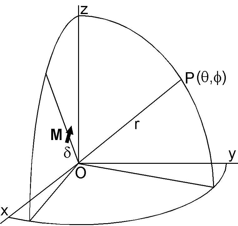
Let the distance vector \({\bf r}\) and the displacement vector \(\boldsymbol{\delta}\) be in the orthogonal coordinates, \begin{eqnarray*} {\bf r} & = & (x, y, z) = (r\sin\theta\cos\phi, r\sin\theta\sin\phi, r\cos\theta), \\ \boldsymbol{\delta} & = & (x_c, y_c, z_c). \end{eqnarray*} The potential \(W\) given by \eqref{eq01} becomes, \[ W = \frac{\mu_0}{4\pi}\left(\frac{M_x x}{r^3} + \frac{M_y y}{r^3} +\frac{M_z z}{r^3}\right). \] Then the first order term of the Taylor expansion becomes as the followings. \begin{eqnarray*} -\boldsymbol{\delta}\cdot\nabla W & = & -(x_c, y_c, z_c)\cdot \\ & & \frac{\mu_0}{4\pi}\left(-\frac{3M_x x^2}{r^5} + \frac{M_x}{r^3} - \frac{3M_y xy}{r^5} - \frac{3M_z xz}{r^5},\right. \\ & & -\frac{3M_x xy}{r^5} - \frac{3M_y y^2}{r^5} + \frac{M_y}{r^3} - \frac{3M_z yz}{r^5}, \\ & & \left.-\frac{3M_x xz}{r^5} - \frac{3M_y yz}{r^5} - \frac{3M_z z^2}{r^5} + \frac{M_z}{r^3}\right), \\ & = & \frac{\mu_0}{4\pi}\left(\frac{M_x x_c(3x^2-r^2)}{r^5} + \frac{3M_y x_c xy}{r^5} + \frac{3M_z x_c xz}{r^5}\right. \\ & & + \frac{3M_x y_c xy}{r^5} + \frac{M_y y_c(3y^2-r^2)}{r^5} + \frac{3M_z y_c yz}{r^5} \\ & & \left. + \frac{3M_x z_c xz}{r^5} + \frac{3M_y z_c yz}{r^5} + \frac{M_z z_c(3z^2-r^2)}{r^5}\right), \\ & = & \frac{\mu_0}{4\pi r^3}\left(M_x x_c(3\sin^2\theta\cos^2\phi-1) + 3M_y x_c\sin^2\theta\cos\phi\sin\phi\right. \\ & & + 3M_z x_c\sin\theta\cos\theta\cos\phi + 3M_x y_c\sin^2\theta\cos\phi\sin\phi \\ & & + M_y y_c(3\sin^2\theta\sin^2\phi-1) + 3M_z y_c\sin\theta\cos\theta\sin\phi \\ & & + 3M_x z_c\sin\theta\cos\theta\cos\phi + 3M_y z_c\sin\theta\cos\theta\sin\phi \\ & & + \left.M_z z_c(3\cos^2\theta-1)\right). \end{eqnarray*} This expression is further altered by using the following formulas. \begin{align*} & P_2^0(\cos\theta) = (1/2)(3\cos^2\theta - 1), \quad P_2^1(\cos\theta) = \sqrt{3}\cos\theta\sin\theta, \\ & P_2^2(\cos\theta) = (\sqrt{3}/2)\sin^2\theta, \quad \sqrt{3}P_2^2(\cos\theta) - 1 = -P_2^0(\cos\theta), \\ & \cos^2\phi = (1+\cos 2\phi)/2, \quad \sin^2\phi = (1-\cos 2\phi)/2, \quad \cos\phi\sin\phi = \sin 2\phi/2. \end{align*} Using these formulas and writing \(P_n^m(\cos\theta)\) as \(P_n^m\) for brevity, \begin{eqnarray*} -\boldsymbol{\delta}\cdot\nabla W & = & \frac{\mu_0}{4\pi r^3}\left((2M_z z_c - M_x x_c - M_y y_c)P_2^0\right. \\ & & + \sqrt{3}(M_z x_c + M_x z_c)P_2^1\cos\phi + \sqrt{3}(M_z y_c + M_y z_c)P_2^1\sin\phi \\ & & + \left.\sqrt{3}(M_x x_c - M_y y_c)P_2^2\cos 2\phi + \sqrt{3}(M_y x_c + M_x y_c)P_2^2\sin 2\phi\right). \end{eqnarray*} This equation is compared with \(n\)=2 terms of spherical harmonics expression of the potential of the geomagnetic field (equation (1) of previous page); \[ W_2 = a\left(\frac{a}{r}\right)^3\left(g_2^0 P_2^0 + g_2^1 P_2^1\cos\phi + h_2^1 P_2^1\sin\phi + g_2^2 P_2^2\cos 2\phi + h_2^2 P_2^2\sin 2\phi\right). \] Hence, when the dipole \({\bf M}\) at the earth's center is displaced by \(\boldsymbol{\delta}\), the next \(n\)=2 terms appears. \begin{eqnarray} g_2^0 & = & \frac{\mu_0}{4\pi a^4}(2M_z z_c - M_x x_c - M_y y_c) = \frac{1}{a}(2g_1^0 z_c - g_1^1 x_c - h_1^1 y_c), \nonumber \\ g_2^1 & = & \frac{\mu_0}{4\pi a^4}\sqrt{3}(M_z x_c + M_x z_c) = \frac{\sqrt{3}}{a}(g_1^0 x_c + g_1^1 z_c), \nonumber \\ h_2^1 & = & \frac{\mu_0}{4\pi a^4}\sqrt{3}(M_z y_c + M_y z_c) = \frac{\sqrt{3}}{a}(g_1^0 y_c + h_1^1 z_c), \label{eq03} \\ g_2^2 & = & \frac{\mu_0}{4\pi a^4}\sqrt{3}(M_x x_c - M_y y_c) = \frac{\sqrt{3}}{a}(g_1^1 x_c - h_1^1 y_c), \nonumber \\ h_2^2 & = & \frac{\mu_0}{4\pi a^4}\sqrt{3}(M_y x_c + M_x y_c) = \frac{\sqrt{3}}{a}(h_1^1 x_c + g_1^1 y_c). \nonumber \\ \end{eqnarray}
It is of interest to find \(\boldsymbol{\delta}\) from the observed Gauss coefficients by using \eqref{eq03}. As there are more equations than the unknowns in \eqref{eq03}, the least squares method should be used to determine \((x_c,y_c,z_c)\), which was first carried out by Adolf Schmidt in 1930's (→ details are here). Using Schmidt's formulas, the displacement in the unit of km for the year 2015 is as the followings. \[ \delta = 576.7, \quad x_c = -399.9, \quad y_c = 351.7, \quad z_c = 221.3. \] The displacement amounts to about 9% of the earth's radius.
Second order term of the Taylor expansion \eqref{eq02} causes appearance of Gauss coefficients of \(n\)=3. They are derived similarly by manipulating \((1/2!)\boldsymbol{\delta}\cdot\nabla(\boldsymbol{\delta}\cdot\nabla W)\) with further more laborious practice. Here, only the results are shown; \begin{eqnarray*} g_3^0 & = & \frac{3}{2a^2}\left(g_1^0(2z_c^2 - x_c^2 - y_c^2) - 2g_1^1 x_c z_c - 2h_1^1 y_c z_c\right), \\ g_3^1 & = & \frac{3}{2\sqrt{6}a^2}\left(8g_1^0 x_c z_c + g_1^1(4z_c^2 - 3x_c^2 - y_c^2) - 2h_1^1 x_c y_c\right), \\ h_3^1 & = & \frac{3}{2\sqrt{6}a^2}\left(8g_1^0 y_c z_c - 2g_1^1 x_c y_c + h_1^1(4z_c^2 - x_c^2 - 3y_c^2)\right), \\ g_3^2 & = & \frac{15}{2\sqrt{15}a^2}\left(g_1^0(x_c^2 - y_c^2) + 2g_1^1 x_c z_c - 2h_1^1 y_c z_c\right), \\ h_3^2 & = & \frac{15}{\sqrt{15}a^2}\left(g_1^0 x_c y_c + g_1^1 y_c z_c + h_1^1 z_c x_c\right), \\ g_3^3 & = & \frac{15}{2\sqrt{10}a^2}\left(g_1^1(x_c^2 - y_c^2) - 2h_1^1 x_c y_c\right), \\ h_3^3 & = & \frac{15}{2\sqrt{10}a^2}\left(2g_1^1 x_c y_c + h_1^1(x_c^2 - y_c^2)\right). \end{eqnarray*}
References:
- James, R. W., & D. E. Winch, The eccentric dipole, Pure Applied Geophys., 66, 77-86, 1967.