Thermoremanent magnetization of single-domain grains: Neel diagram
Graphical representation was also presented in Neel (1949) to visualize the concept of blocking in the TRM acquisition of SD grains. As shown in the previous page (equations (1), (3), (4), and (6)), relaxation time \(\tau\) is given by, \begin{eqnarray} \frac{1}{\tau} & = & \frac{1}{\tau_{12}} + \frac{1}{\tau_{21}} = A\exp\left(-\frac{\Delta E_{12}}{kT}\right) + A\exp\left(-\frac{\Delta E_{21}}{kT}\right), \nonumber \\ & = & A\exp\left[-\frac{\mu_0 VM_s H_K}{2kT}\left(1+\frac{H}{H_K}\right)^2\right] \nonumber \\ & & \qquad\qquad + A\exp\left[-\frac{\mu_0 VM_s H_K}{2kT}\left(1-\frac{H}{H_K}\right)^2\right]. \label{eq01} \end{eqnarray} We first derive an approximate expression of this equation.
Case for a small \(H\)
For a small \(H\), such as a geomagnetic field, (1) is approximated as, \begin{equation} \frac{1}{\tau} \approx 2A\exp\left(-\frac{\mu_0 VM_s H_K}{2kT}\right), \quad \frac{\mu_0 VM_s}{kT}H \ll 1. \label{eq02} \end{equation} This is obvious for \(H\) = 0. For a small nonzero \(H\), the derivation is as the followings. First, the second order term \((H/H_K)^2\) in (1) is omitted as, \begin{eqnarray*} \frac{1}{\tau} & \approx & A\exp\left[-\frac{\mu_0 VM_s H_K}{2kT}\left(1+\frac{2H}{H_K}\right)\right] + A\exp\left[-\frac{\mu_0 VM_s H_K}{2kT}\left(1-\frac{2H}{H_K}\right)\right], \\ & = & A\exp\left(-\frac{\mu_0 VM_s H_K}{2kT}\right)\left[\exp\left(-\frac{\mu_0 VM_s}{kT}H\right) + \exp\left(\frac{\mu_0 VM_s}{kT}H\right)\right]. \end{eqnarray*} Using \(e^x \approx 1+x\) \((|x|\ll 1)\), the term \([\cdots]\) becomes 2 and hence (2) is obtained. \(H\) satisfying the condition of (2) is estimated for a spherical magnetite grain with a diameter 50 nm at a high temperature 500°C as: \[ \mu_0 H \ll \frac{1.3807\times 10^{-23}\times 773}{(\pi/6)\times(50\times 10^{-9})^3\times 480\times 10^3} = 3.4\times 10^{-4}\ \mathrm{T} = 340\ \mathrm{\mu T}. \] Hence, (2) can be applied to the blocking process in the geomagnetic field of ~50 μT.
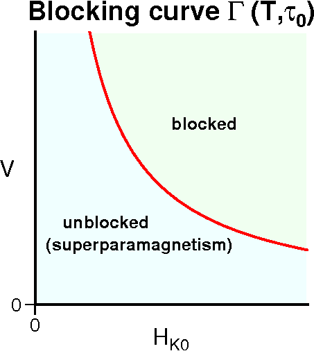
Rewriting equation (2) as, \[ \exp\left(\frac{\mu_0 V M_s H_K}{2kT}\right) = 2A\tau, \] and, \[ VH_K = \frac{2kT\log(2A\tau)}{\mu_0 M_s}. \] Introducing temperature variation \(F(T)\) of \(M_s\) and \(H_K\) as, \[ M_s = M_{s0}F(T),\quad H_K = (N_p-N_l)M_s = H_{K0}F(T), \] where \(M_{s0}\) and \(H_{K0}\) are those at the room temperature \(T_0\), the above relation is expressed as, \begin{equation} VH_{K0} = \frac{2kT\log(2A\tau)}{\mu_0 M_{s0}F^2(T)}. \label{eq03} \end{equation} Taking \(V\) and \(H_{K0}\) as ordinate and abscissa, respectively, (3) forms a hyperbola in which \(T\) and \(\tau\) are the parameters to define its shape. The curve, denoted here as \(\Gamma(T,\tau)\), defines a series of grains \((V,H_{K0})\) which have the same relaxation time \(\tau\) at temperature \(T\). Suppose \(T\) is fixed at a certain temperature, if the curve moves toward upper-right direction by a small distance, the term \(\log(2A\tau)\) increases by a small amount because \(T\) is supposed to be constant, leading into exponential increase of \(\tau\). Conversely, if the curve moves toward lower-left direction by a small distance, \(\tau\) drastically decreases. Hence, if \(\tau\) is taken as an observation time \(\tau_0\) at \(T\) (characteristic time of cooling), curve \(\Gamma(T,\tau_0)\) is a boundary which divides the \(V\)-\(H_{K0}\) plane into the upper-right area in which SD grains are blocked and the lower-left area in which the grains are unblocked (superparamagnetism) as shown in the above figure.
Consider a TRM acquisition process. At a high temperature \(T_1\), \(\Gamma(T_1,\tau_0)\) is at the far up-right area and only the grains of large values of \(VH_{K0}\) are blocked. As the temperature is lowered to \(T_2\), the curve moves toward lower-left direction to \(\Gamma(T_2,\tau_0)\) and the grains in the area between \(\Gamma(T_1,\tau_0)\) and \(\Gamma(T_2,\tau_0)\) are blocked. Hence, the curve \(\Gamma(T,\tau_0)\) is called a blocking curve. The remanence blocked in such a way between \(T_i\) and \(T_{i+1}\) is called a partial TRM (pTRM). When \(T\) is lowered to the room temperature \(T_0\), the blocking curve \(\Gamma(T_0,\tau_0)\) is at the low-left area and the total remanence blocked (TRM) is the sum of pTRMs.
Blocking curves \(\Gamma(T,\tau_0)\) for several temperatures are plotted in the figure below in which grain diameter \(d\) is taken as the ordinate instead of volume \(V\). Calculation was made with \(A\) = 109 s-1 and \(\tau_0\) = 10 s. Temperature variation \(F(T)\) of \(M_s\) and \(H_K\) was supposed as, \begin{equation} F(T) = \sqrt{(T_C - T)\left/(T_C - T_0)\right.}, \label{eq04} \end{equation} where \(T_C\) is the Curie temperature (580°C) of magnetite.
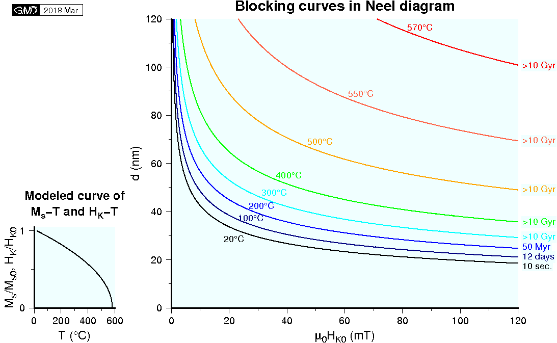
Grains which were blocked at a high temperature \(T\), i.e. grains along the blocking curve \(\Gamma(T,\tau_0)\), would have an extremely large relaxation time \(\tau'\) when cooled to the room temperature \(T_0\). Hence, the blocking curve \(\Gamma(T,\tau_0)\) is also the curve of equal relaxation time at \(T_0\), \(\Gamma(T_0,\tau')\), which indicates how the blocked remanence is stable depending on \(\tau'\). In the figure, \(\tau'\) is indicated at the right side of each curve. It should be noted that the relaxation time \(\tau'\) of ~50 My for the remanence blocked at 200°C is not very long in terms of geological time scale. This is the reason for that the remanence component with the blocking temperature \(T_B\) lower than ~200°C might not be a primary origin at least for the old rocks, say of Cretaceous or older ages. Conversely, there should be no concern about the remanence component with \(T_B\) higher than ~300°C even for very old rocks of Precambrian because \(\tau'\) is longer than ~10 Gy.
Case for a large \(H\)
Another approximation of equation (1) for a large \(H\) was proposed by Neel (1949) as, \begin{equation} \frac{1}{\tau} \approx \frac{1}{\tau_{21}} = A\exp\left[-\frac{\mu_0 VM_s H_K}{2kT}\left(1-\frac{H}{H_K}\right)^2\right], \quad \frac{\mu_0 VM_s}{kT}H > 4. \label{eq05} \end{equation} This is derived from the fact that rotation 1→2 seldom occurs when a large positive \(H\) is applied, i.e. \(\tau_{12}\gg\tau_{21}\) (1/\(\tau_{12}\) \(\ll\) 1/\(\tau_{21}\)). Let the relaxation times be compared by the ratio; \begin{eqnarray*} \frac{1}{\tau_{12}}\left/\frac{1}{\tau_{21}}\right. & = & \exp\left[-\frac{\mu_0 VM_s H_K}{2kT}\left(1+\frac{H}{H_K}\right)^2\right] \left/\exp\left[-\frac{\mu_0 VM_s H_K}{2kT}\left(1-\frac{H}{H_K}\right)^2\right]\right., \\ & = & \exp\left[-\frac{\mu_0 VM_s H_K}{2kT}\left(\left(1+\frac{H}{H_K}\right)^2 - \left(1-\frac{H}{H_K}\right)^2\right)\right], \\ & = & \exp\left(-\frac{2\mu_0 VM_s}{kT}H\right). \end{eqnarray*} The ratio for the condition of (5) gives \(e\)-8 = 0.0003, and hence approximated expression (5) of 1/\(\tau\) is justified. The field \(H\) which satisfies this condition for the spherical magnetite grain with \(d\) = 50 nm at \(T_0\) is, \[ \mu_0 H > \frac{4\times 1.3807\times 10^{-23}\times 293}{(\pi/6)\times(50\times 10^{-9})^3\times 480\times 10^3} = 5.15\times 10^{-4}\ \mathrm{T} \approx 0.5\ \mathrm{mT}. \] Hence, (5) can be a theoretical basis for the normal paleomagnetic experiments using DC or AC magnetic fields which are usually larger than a few mT.
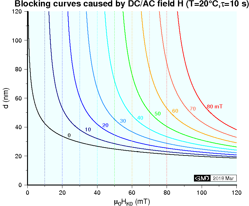
Rewriting (5) as, \[ \exp\left[\frac{\mu_0 VM_s H_K}{2kT}\left(1-\frac{H}{H_K}\right)^2\right] = A\tau, \] and using temperature variation \(F(T)\) of \(M_s\) and \(H_K\), \begin{equation} VH_{K0}\left(1-\frac{H}{H_{K0}F(T)}\right)^2 = \frac{2kT\log(A\tau)}{\mu_0 M_{s0}F^2(T)}. \label{eq06} \end{equation} If a characteristic time \(\tau_0\) (observation time) is taken for \(\tau\), (6) is a blocking curve \(\Gamma(T,H,\tau_0)\) on \(V\)-\(H_{K0}\) plane when \(H\) is applied at temperature \(T\). Shape of the curve is similar to a hyperbola but has a vertical asymptote at \(H_{K0}\) = \(H\). Substituting (4) to \(F(T)\) and setting \(A\) = 109 s-1, \(\tau_0\) = 10 s, and \(T\) = \(T_0\) = 293 K, blocking curves \(\Gamma(T_0,H,\tau_0)\) for \(H\) of several magnitudes are shown in the figure below. Considering a curve of a certain \(H\), grains in the lower-left area are unblocked (superparamagnetism), i.e. magnetizations are rotated to the direction of \(H\), while those in the upper-right area are blocked, i.e. magnetizations are not affected by \(H\). When \(H\) is reduced to zero, magnetization of the grains in the lower-left area become blocked with the direction of \(H\), which is the isothermal remanent magnetization (IRM). If similar procedure is carried out with AC field \(\tilde H\), the magnetizations are randomized, which is the alternating field (AF) demagnetization. It is noted that application of \(H\) can unblock magnetizations whose microcoercivity \(H_{K0}\) is larger than the applied field \(H\) if their volumes are small enough. This is the result of input of thermal energy even at the room temperature.
Importance of thermal demagnetization
As a routine procedure of paleomagnetic measurements, stepwise demagnetization is carried out to the remanence of rock samples. This is not only to remove noise components (magnetic cleaning) of NRM (natural remanent magnetization) but also to define the vector of the characteristic remanence (ChRM) which was acquired during the initial rock formation. In stepwise thermal demagnetization (THD), a rock sample is heated to a certain temperature \(T_i\) and cooled to \(T_0\) in zero-field space. This process is repeated to successively higher temperatures \(T_{i+1}\), \(T_{i+2}\), \(\cdots\), until over \(T_C\) is attained. Curve \(\Gamma(T,\tau_0)\) is now unblocking curve and the unblocking temperature \(T_{UB}\) is equal to the blocking temperature \(T_B\) as long as the remanence is carried by SD grains. In the course of THD, curve \(\Gamma(T,\tau_0)\) sweeps the \(V\)-\(H_{K0}\) plane from lower-left to upper-right areas and randomizes the grains' magnetizations it passes through.
Procedure of stepwise alternating field demagnetization (AFD) is similar to THD; alternating field with a peak field \(H_i\) is applied to the sample and its amplitude is gradually decreased to zero under zero-field space. This process is repeated to successively higher peak fields, \(H_{i+1}\), \(H_{i+2}\), \(\cdots\). In the course of AFD, the unblocking curve \(\Gamma(T_0,H,\tau_0)\) sweeps the \(V\)-\(H_{K0}\) plane from left to right and randomizes the magnetizations it passes through.
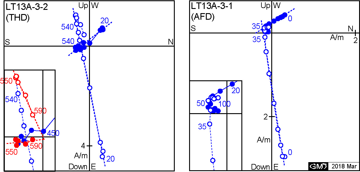
As an experimental procedure, AFD is easier and quicker than THD. Nevertheless, it is advised to apply THD to at least one sample per site. This is because in THD the unblocking curve sweeps along an inclined direction on \(V\)-\(H_{K0}\) plane, exactly reversed way as TRM acquisition, while in AFD it moves in different way of horizontal direction. Both methods correctly depict the vector of ChRM for the NRM which consists of a single component. However, THD is often superior to AFD in the case of NRM which contains two or more components. For example, if NRM contains pTRMs acquired in different directions of \(H\) in different \(T\) ranges, discrimination of them is often easier in THD than AFD, although this depends on the actual grain distribution on the \(V\)-\(H_{K0}\) plane. Figure below shows a case of Icelandic lava flow in which the original remanence was partially remagnetized by the heat from the overlying lava flow (Tanaka & Yamamoto, 2016). In the vector diagram of THD, the survived original remanence in reversed direction is clearly defined over 550°C (red circles in the inset) while it is blurred in the diagram of AFD.
References:
- Neel, L., Theorie du trainage magnetique des ferromagnetiques en grains fins avec applications aux terres cuites, Ann. Geophys., 5, 99--136, 1949.
- Tanaka, H., and Y. Yamamoto, Palaeointensities from Pliocene lava sequences in Iceland: emphasis on the problem of Arai plot with two linear segments, Geophys. J. Int., 205, 694-714, 2016. (→ doi:10.1093/gji/ggw031)