Thermoremanent magnetization of single-domain grains: Magnetic hysteresis of a single-domain grain
Magnetic potential energy and magnetostatic energy
Consider a small magnetic grain which has a uniform magnetization \({\bf M}\). Such a grain is called a single-domain (SD) grain compared to a multidomain (MD) grain which consists of two or more parts with different directions of magnetization. When a magnetic field \({\bf H}\) is applied to the SD grain, the magnetic potential energy \(E_m\) is \begin{equation} E_m = -\mu_0V{\bf M}\cdot {\bf H}, \label{eq01} \end{equation} where \(V\) is the volume of the grain. Due to this energy, the magnetization \({\bf M}\) tends to align to \({\bf H}\) so that \(E_m\) becomes the minimum.
On the other hand, magnetic grains have magnetic anisotropy which leads to preferred direction(s) of \({\bf M}\), called easy axis(es), so that the magnetic anisotropy energy becomes the minimum. Magnetic anisotropy arises from grain shape, crystal structure, and the state of stress within the crystal. Hereafter, we consider only the shape anisotropy which is often the most dominant in SD grains.
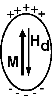
Let a SD grain with spheroidal shape has magnetization along the axis of elongation (easy axis). Even if no external magnetic field is applied, there exists an internal field inside the grain, which is the demagnetizing field \({\bf H_d}\). \({\bf H_d}\) arises from the surface magnetic poles induced by \({\bf M}\). \({\bf H_d}\) points to the opposite direction to \({\bf M}\), given by, \[ {\bf H_d} = -N{\bf M}, \] where \(N\) is the demagnetizing factor. As the demagnetizing field \({\bf H_d}\) interacts with \({\bf M}\), another magnetic energy emerges following equation (1). However, as \({\bf H_d}\) is induced by \({\bf M}\) itself, the energy equation should be derived in terms of accumulation of a small increase in energy \(dE\) caused by a small increase in magnetization \(dM\); \[ dE = -\mu_0 V dM H_d = \mu_0 V N M dM. \] Integrating this equation, \[ E = {\scriptsize \frac{1}{2}}\mu_0 V N M^2. \] This energy is called magnetostatic (self-)energy or demagnetizing energy and the formula for a general case is, \begin{equation} E_d = {\scriptsize \frac{1}{2}}\mu_0 V{\bf M}\cdot{\bf N}\cdot{\bf M}, \label{eq02} \end{equation} where \({\bf N}\) is the demagnetizing tensor (Dunlop & Ozdemir 1997). The magnetostatic energy \(E_d\) is the cause of the shape anisotropy of SD grains.
Rotation of magnetization under a magnetic field
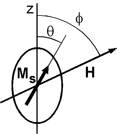
Now consider a SD grain of volume \(V\) with the shape of prolate spheroid. Let the SD grain has a spontaneous magnetization \({\bf M_s}\) along the long (easy) axis which is taken as \(+z\) axis. Right figure shows the \({\bf M_s}\) which deflected from the \(z\)-axis by an angle \(\theta\) when \({\bf H}\) is applied at an angle \(\phi\). Using equation (2), the magnetostatic energy \(E_d\) of the SD grain is given by, \[ E_d = {\scriptsize \frac{1}{2}}\mu_0 V({M_s}_x,{M_s}_y,{M_s}_z) \left(\begin{array}{ccc} N_p & 0 & 0 \\ 0 & N_p & 0 \\ 0 & 0 & N_l \end{array}\right) \left(\begin{array}{c} {M_s}_x \\ {M_s}_y \\ {M_s}_z \end{array}\right), \] where \(N_l\) and \(N_p\) are the demagnetizing factors along the \(z\) (long) and \(x\), \(y\) (perpendicular) axes, respectively. Performing the multiplication, \(E_d\) is simplified to, \[ E_d = {\scriptsize \frac{1}{2}}\mu_0 V(N_p - N_l)M_s^2\sin^2\theta + {\scriptsize \frac{1}{2}}\mu_0 V N_l M_s^2. \] Using the relation for the demagnetizing factors, \(N_x+N_y+N_z=1\), \(N_p-N_l\) in the first term is given by, \[ N_p - N_l = (1 - N_l)/2 - N_l = (1 - 3N_l)/2. \] Considering that \(N_x = N_y = N_z = \frac{1}{3}\) for a sphere, \(N_p\) > \({1 \over 3}\) and \(N_l\) < \({1 \over 3}\). Hence, \(N_p - N_l\) is positive and \({1 \over 2}\) at the maximum. It is also noted that the second term of the above \(E_d\) is constant to \(\theta\) and can be ignored. Hence, the final expression of \(E_d\) is given by, \begin{equation} E_d = {\scriptsize \frac{1}{2}}\mu_0 V(N_p - N_l)M_s^2\sin^2\theta. \label{eq03} \end{equation} Note that \(E_d\) is always positive and is the minimum at \(\theta=0\) and \(\pi\), making the \(z\)-axis an easy direction for \({\bf M_s}\).
Total magnetic energy \(E_T\) of the SD grain is the sum of the magnetic potential energy \(E_m\) of (1) and the magnetostatic energy \(E_d\) of (3); \begin{equation} E_T = -\mu_0 V M_s H\cos(\phi - \theta) + {\scriptsize \frac{1}{2}}\mu_0 V(N_p - N_l)M_s^2\sin^2\theta. \label{eq04} \end{equation} \(\theta\) which satisfies \(dE_T/d\theta\) = 0 and \(d^2E_T/d\theta^2\) > 0 is the solution for the minimum \(E_T\), i.e., the equilibrium direction of \({\bf M_s}\) for the applied field \({\bf H}\). Hence, equations to be solved are as the followings. \begin{eqnarray} \frac{dE_T}{d\theta} & = & \mu_0 V M_s\left(H\sin(\theta-\phi) + {\scriptsize \frac{1}{2}}(N_p - N_l)M_s\sin 2\theta\right) = 0, \label{eq05} \\ \frac{d^2E_T}{d\theta^2} & = & \mu_0 V M_s\left(H\cos(\theta-\phi) + (N_p - N_l)M_s\cos 2\theta\right) > 0. \label{eq06} \end{eqnarray}
Case of a magnetic field parallel to the easy axis
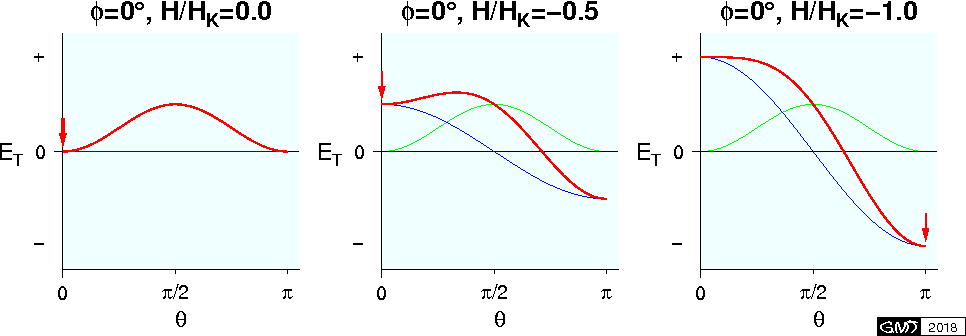
Analytical solutions of equations (5) and (6) are available only for \(\phi=0\) and \(\pi/2\). For \(\phi=0\), the equation \(dE_T/d\theta=0\) is \[ \mu_0 V M_s \sin\theta\left(H + (N_p - N_l)M_s \cos\theta\right) = 0. \] Solutions of this equation are, \begin{eqnarray*} & & 0, \quad \pi, \quad \theta_c = \cos^{-1}(-H/H_K) \quad for \quad |H/H_K| < 1, \\ & & 0, \quad \pi \quad for \quad |H/H_K| \geq 1, \end{eqnarray*} where \(H_K\) is introduced as, \begin{equation} H_K = (N_p - N_l)M_s. \label{eq07} \end{equation} Examining the sign of \(d^2E_T/d\theta^2\), it is shown that, for \(|H/H_K|\) < 1, the local minimum of \(E_T\) occurs at \(\theta=0\) and \(\pi\), and the maximum at \(\theta_c\). For the case of \(|H/H_K|\) ≥ 1, the minimum \(E_T\) is at \(\theta=0\) and \(\pi\) for \(H\) ≥ \(H_K\) and \(H\) ≤ \(-H_K\), respectively. These results indicate that when a small negative field (\(H\) < 0) is applied to \({\bf M_s}\) originally at \(\theta=0\) and its amplitude is gradually increased, \({\bf M_s}\) stays at the original position until \(H\) reaches \(-H_K\), and at that point \({\bf M_s}\) flips to \(\theta=\pi\) direction. This is shown in the following \(E_T\) vs. \(\theta\) curves for three successive \(H\)'s, in which blue, green, and red lines are \(E_m\), \(E_d\), and \(E_T\), respectively. Equilibrium position of \({\bf M_s}\) is also shown by a red arrow.
Magnetic hysteresis curves of a SD grain
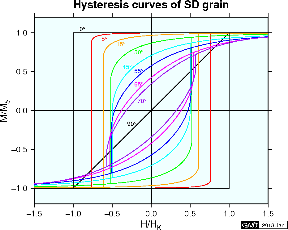
It is noted that once \({\bf M_s}\) flips from \(\theta=0\) to \(\pi\) by applying \(H\) ≤ \(-H_K\), it stays at \(\theta=\pi\) until \(H\) ≥ \(+H_K\) is applied. This phenomenon is called magnetic hysteresis and \(H_K\) given by (7) is a microscopic coercivity (coercive force). Consider a case that we measure \({\bf M}\) along \({\bf H}\) direction, starting at \(+M_s\), while \(H\) is cyclically varied in such a way; \(H=0\) \(\rightarrow\) \(H\) < \(-H_K\) \(\rightarrow\) \(H=0\) \(\rightarrow\) \(H\) > \(+H_K\) \(\rightarrow\) \(H=0\). In such a measurement a rectangular \(M\) vs. \(H\) curve is obtained. In general, such a curve is called a magnetic hysteresis curve (loop) and its shape depends on \(\phi\) as shown below. It is known that the smallest \(H\) which makes \({\bf M_s}\) to flip is \(H_K/2\) for \(\phi=\pi/4\).
Case of a magnetic field perpendicular to the easy axis
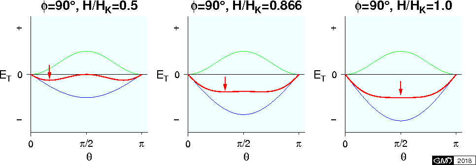
Another analytical solution for the equations (5) and (6) is the case of \(\phi=\pi/2\), in which \(M\) vs. \(H\) relation is linear as shown in the above figure. This is easily shown as the followings. \(\theta\) for \(dE_T/d\theta=0\) and \(d^2E_T/d\theta^2\) > \(0\) is \[ \theta_c = \sin^{-1}(H/H_K) \quad for \quad |H/H_K| \leq 1. \] As \(M\) is measured along \({\bf H}\) direction, \[ M = M_s\cos\left({\scriptsize \frac{\pi}{2}} - \theta_c\right) = M_s\sin\theta_c = (M_s/H_K)H. \] \(E_T\) vs. \(\theta\) curves for \(\phi=\pi/2\) are shown below for three cases of \(H\), in which blue, green, and red lines are \(E_m\), \(E_d\), and \(E_T\), respectively, and a red arrow indicates the equilibrium position of \({\bf M_s}\).
Magnetic hysteresis curve of randomly oriented SD grains
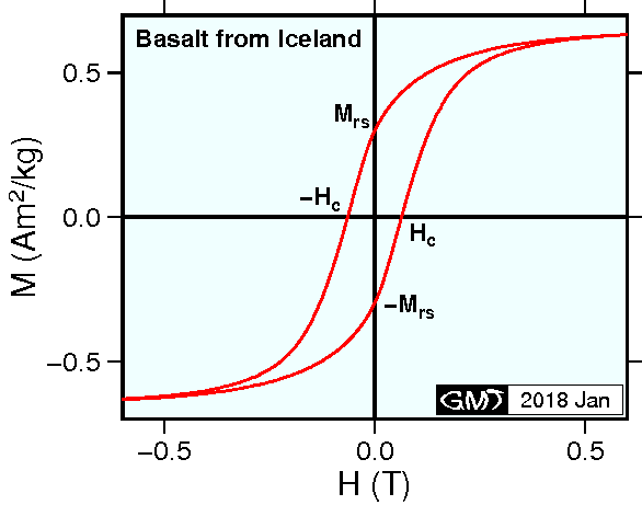
For a mass of randomly oriented SD grains, the bulk \(M\) vs. \(H\) curve is the average of the curves for various values of \(\phi\). \(M\) vs. \(H\) curve of such material would look like the one shown in the right figure which is the measurement of a basalt sample from Iceland. Magnetic grains contained in this sample seem to be SD grains although those contained in natural rocks are mostly small MD grains called pseudo-single-domain (PSD) grains. In the \(M\) vs. \(H\) curves, the intersection of the curve and the abscissa, i.e. \(H\) which is necessary to reduce \(M\) to zero, is the coercivity (coercive force) \(H_c\). \(H_c\) of a sample of SD grains is the average of those of various \(\phi\) (from \(H_K\) for \(\phi=0\) to \(0\) for \(\phi=\pi/2\)), and it is known that \(H_c\) is about half of the microcoercivity \(H_K\).
The residual remanence at \(H=0\) is called the saturation remanence \(M_{rs}\). \(M_{rs}\) is theoretically half of \(M_s\), which is shown as the following. When \(H\) is reduced from \(H_{max}\) to \(0\), \({\bf M_s}\) of each SD grain stays at the easy axis pointing to the nearest direction of \(H\). Hence, \(M_{rs}\) is estimated as the average of \(M_s\cos\phi\) over the surface of the hemisphere with \(H\) direction at the center, \[ M_{rs} = \left.\int_0^{\pi \over 2} M_s\cos\phi\sin\phi d\phi\right/\int_0^{\pi \over 2} \sin\phi d\phi = {\scriptsize \frac{1}{2}}M_s. \] In fact, \(M_{rs}\) is almost half of \(M_s\) in the measurement of the basalt sample shown in the figure.
References:
- Dunlop, D. J., and O. Ozdemir, Rock Magnetism --- Fundamentals and frontiers ---, 573 pp., Cambridge University Press, Cambridge, 1997.