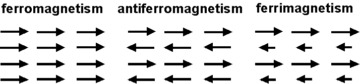
Magnetism of material: Ferromagnetism
Ferromagnetism appears in the material in which magnetic atoms have strong interaction. Due to the interaction, ferromagnetic material shows spontaneous magnetization in the absence of external magnetic field. There are only four elements, Fe, Ni, Co, and Gd, which show ferromagnetism, but there are many compounds with strong magnetization which include one of these elements. Ferromagnetism as a general term refers to strong magnetism. Strictly speaking, ferromagnetism is one type of magnetism which arises from the interaction of atom's magnetic moment as shown in the figure below. Antiferromagnetism is weak magnetism similar to paramagnetism but magnetic susceptibility is smaller. This is because atoms' magnetic moments are less perturbed by thermal energy due to their strong interaction. Ferrimagnetism is mostly similar to ferromagnetism but could show complicated thermal behavior when the magnetic moments with opposite directions have different temperature dependency. All these magnetism become paramagnetic when the temperature exceeds a critical point called Curie temperature (\(T_C\)). Magnetite, Fe3O4, main magnetic mineral in rocks, is ferrimagnetism.
Weiss theory
The strong interaction between atom's magnetic moments is called exchange interaction which is explained only by quantum theory. Nevertheless, basics of ferromagnetism can be understood with introductory physics by using Weiss theory. In the theory, it is supposed that the interaction is caused by a strong internal field \({\bf H_m}\) (molecular field) which is proportional to the magnetization \({\bf M}\) of the material, \begin{equation} H_m = w M, \label{eq01} \end{equation} where \(w\) is a constant. Introducing the same statistical mechanics as used in the theory of paramagnetism, the Boltzmann's factor is given by, \[ \exp\left(\frac{\mu_0 m(H + wM)}{kT}\cos\theta\right). \] Using this factor, \(M\) is given by the same equations as paramagnetism with modified \(\alpha\) as, \begin{eqnarray} M & = &N m L(\alpha), \label{eq02} \\ \alpha & = & \frac{\mu_0 m(H + wM)}{kT}, \label{eq03} \end{eqnarray} where \(L(\alpha)\) is Langevin function. To see the temperature dependency of spontaneous magnetization, here we set \(H=0\). From (3) with \(H=0\), \(M\) is given by, \begin{equation} M = \frac{kT}{\mu_0 m w}\alpha. \label{eq04} \end{equation} Giving \(T\) as a parameter, \(\alpha\) and \(M\) can be determined by solving equations (2) and (4). The solution is given as an intersection point of curves of equations (2) (Langevin function) and (4) (straight line) as shown in the figure below. As temperature \(T\) increases from 0 K, the intersection point moves on the Langevin function curve from the upper right toward the lower left. At the critical point of Curie temperature \(T_C\), the intersection point reaches to the origin. Beyond the Curie temperature, molecular field \(H_m\), or \(wM\), disappears and ferromagnetism turns to paramagnetism.
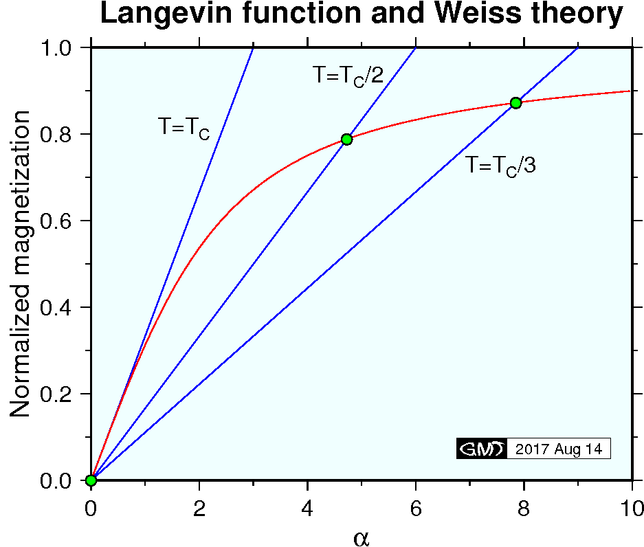
At the Curie temperature \(T_C\), tangents of the two curves (2) and (4) are equal. Approximating \(L(\alpha) \sim \alpha/3\) for small \(\alpha\) and equating the gradients of (2) and (4) at \(\alpha=0\), the next relation is obtained, \[ \frac{N m}{3} = \frac{k T_C}{\mu_0 m w}. \quad (\alpha \ll 1) \] From this relation, the constant \(w\) is obtained as, \begin{equation} w = \frac{3 k T_C}{\mu_0 N m^2}. \label{eq05} \end{equation} Substituting (5) to (4), \begin{equation} M = \frac{N m}{3} \frac{T}{T_C} \alpha. \label{eq06} \end{equation} Introducing normalized variables \(M^*=M/Nm\) and \(T^*=T/T_C\), (2) and (6) are given as, \begin{eqnarray} M^* & = & L(\alpha) \label{eq07} \\ M^* & = & \frac{T^*}{3} \alpha \label{eq08} \end{eqnarray} Although analytical solution for these equations is unavailable, it is easy to solve numerically by using standard root finding routines (ex., Press et al. 1992). Figure below shows the solution of the \(M^*\)-\(T^*\) curve (red line). Measured data of Ni (blue line) for the temperature range higher than the room temperature is also shown.
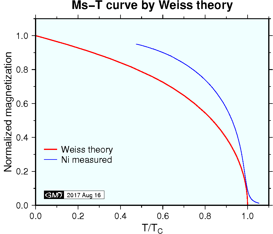
In the figure above, apart from lack of low temperature data in the measurement of Ni, discrepancy of the theoretical and experimental curves is not small. It is known that the Weiss theory is improved by introducing quantum mechanics and shows excellent agreement with measurements (Chikazumi, 1964). Note that the theoretical curve is calculated with \(H\) = 0 while measurement of Ni was made under a strong field of \(B\) = 1 T. Hence, paramagnetic behavior is recognized in the temperatures over \(T_C\).
If \(T_C\) is known, \(w\) is calculated using (5) and then \(H_m\) is estimated by (1). For the case of Fe, molecular weight is 55.8 g and density is 7.87 g/cm3. Hence, \[ N = \frac{6.022\times 10^{23}}{55.8/7.87} = 8.49\times 10^{22}\ \mathrm{cm^{-3}} = 8.49\times 10^{28}\ \mathrm{m^{-3}}. \] As \(T_C\) is 1044 K and \(m\) is 2.2 \(m_B\) (different from Fe ions), using (5) \(w\) is calculated as, \[ w = \frac{3(1.3807\times10^{-23})(1044)} {(4\pi\times10^{-7})(8.49\times10^{28})(2.2\times9.273\times10^{-24})^2} = 974. \] Using these values, (1) gives \(H_m\) as, \[ H_m = wM = wNm = 974(8.49\times10^{28})(2.2\times9.273\times10^{-24}) = 1.69\times10^{9}\ \mathrm{A/m}. \] This is a huge field (\(B\) = 2120 T) which is impossible to create artificially and is explained only by the exchange interaction in quantum mechanics.
References:
- Chikazumi, S., Physics of Magnetism, 554 pp., John Wiley, New York, 1964.
- Press, W. H., S. A. Teukolsky, W. T. Vetterling, and B. P. Flannery, Numerical Recipes in C: The Art of Scientific Computing (Second Edition), 994 pp., Cambridge University Press, Cambridge 1992.