 Statistical Tests: Test of a common mean direction; tmeandir
Program "tmeandir" tests whether two or more groups of unit vectors, distributed in the Fisher distribution, share a common mean direction. It is mainly used in the reversals test of two distributions of paleomagnetic directions in which the reversed directions should be inverted by 180°. The program is also aimed at to test whether three or more site-mean paleodirections share a common mean direction.
Two groups with equal population precision parameters \(\kappa_1=\kappa_2\)
Consider two distributions of unit vectors. Let the data number and the resultant vectors of groups 1 and 2 be denoted as \(N_1\) and \(N_2\), and \({\bf R_1}\) and \({\bf R_2}\), respectively, and those for the sum of all distinct vectors as \(N=N_1+N_2\) and \({\bf R=R_1+R_2}\). Null hypothesis assumed here is,
Under this null hypothesis, Watson (1956) showed that the following statistic, \[ F = (N-2)\frac{R_1 + R_2 - R}{N - R_1 - R_2}, \] is distributed as a \(F\) distribution with the degrees of freedom, \(\nu_1\)=2 and \(\nu_2\)=2(\(N\)-2), if the two populations share an equal precision parameter. Taking the significance level of \(\alpha\), the null hypothesis is rejected if the observed \(F\) exceeds the upper \(\alpha\) point. Although this theorem is based on a very difficult theory, intuitive interpretation is as the followings. Consider two mean directions with a large difference angle but both have small errors, which are considered not to have a common mean direction. In such a case, \(R_1+R_2\) is much larger than \(R\) while \(N\) is quite close to \(R_1+R_2\), and hence the statistic \(F\) will be large, exceeding the critical value corresponding to the significance level.
McFadden & Lowes (1981) updated the above theorem which was adopted in the program "tmeandir". When the two populations share a common precision parameter, \(\kappa_1=\kappa_2\), the statistic is given by \begin{equation} F = (N-2)\frac{R_1 + R_2 - R^2/(R_1 + R_2)}{2(N - R_1 - R_2)}, \label{eq01} \end{equation} which is distributed as a \(F\) distribution with degrees of freedom, \begin{equation} \nu_1 = 2, \quad \nu_2 = 2(N - 2). \label{eq02} \end{equation} The null hypothesis of a common mean direction is rejected if the observed \(F\) exceeds the upper \(\alpha\) point \(F_{\alpha,2,2(N-2)}\). Using the relation of \({\bf R}\) and the difference angle \(\gamma\) between \({\bf R_1}\) and \({\bf R_2}\), \[ R^2 = R_1^2 + R_2^2 + 2 R_1 R_2 \cos\gamma, \] the critical difference angle \(\gamma_c\) corresponding to \(F_{\alpha,2,2(N-2)}\) is obtained from \eqref{eq01} as, \begin{equation} \cos\gamma_c = 1 - \frac{(N-R_1-R_2)(R_1+R_2)}{(N-2)R_1R_2}F_{\alpha,2,2(N-2)}. \label{eq03} \end{equation}
Before the test of a common mean direction is carried out, it is necessary to test whether the two populations share a common precision parameter. Under the null hypothesis of \(\kappa_1=\kappa_2\), using the best estimates \(k_1\) and \(k_2\) of \(\kappa_1\) and \(\kappa_2\), the statistic \begin{equation} F = \frac{k_1}{k_2}, \label{eq04} \end{equation} is distributed as a \(F\) distribution with the degrees of freedom, \begin{equation} \nu_1 = 2(N_2-1), \quad \nu_2 = 2(N_1-1). \label{eq05} \end{equation} Note that the relation of \(\nu_1\) and \(\nu_2\) to \(N_1\) and \(N_2\) is reversed with a factor of 2 from the case of variances described in the previous page. In actual calculation, the larger one of \(k_1\) and \(k_2\) is taken as the numerator of \eqref{eq04} so that \(F\) is always larger than unity (as is the test for variances in the previous page). If the statistic \(F\) obtained from the observation is smaller than the upper \(\alpha/2\) points, it is considered that \(\kappa_1\) and \(\kappa_2\) are not inconsistent with the common precision parameter, and hence proceeds to the test of a common mean direction described above. Otherwise, another method for unequal \(\kappa\) is used.
Two or more groups regardless of equality in population \(\kappa\)
McFadden & Lowes (1981) also developed a test of a common mean direction for three groups when they share a common \(\kappa\). In such a case, program "tmeandir" uses this method for three groups, although description of the theory is omitted here.
When the population precision parameters of two or more groups are unequal, program "tmeandir" uses a method proposed by G.S. Watson in 1983. This method can be applicable to the cases of two or multi groups regardless of their sharing a common \(\kappa\). The method is described in McFadden & McElhinny (1990) and also at p.211 of Fisher et al. (1987).
Consider \(m\) groups of unit vectors and let \(N\), \(k\) and \({\bf R}\) for \(i\)-th group be denoted as \(N_i\), \(k_i\), and \({\bf R_i}\), where \(i=1,\cdots,m\). Statistics used in the method are, a weighted sum \(S_r\) of the lengths of the resultant vectors, \[ S_r = k_1 R_1 + k_2 R_2 + \cdots + k_m R_m, \] and a weighted vector sum \({\bf R_w}\) of the resultant vectors, \[ {\bf R_w} = k_1{\bf R_1} + k_2{\bf R_2} + \cdots + k_m{\bf R_m}. \] Watson showed that the statistic, \begin{equation} V = 2(S_r - R_w), \label{eq06} \end{equation} is approximately distributed as a \(\chi^2\) distribution with a degrees of freedom \(2(m-1)\), only when all sample sizes are large (\(N_i ≥ 25\)). Nevertheless, as proposed in McFadden & McElhinny (1990), this method can be applied to the samples of small size if computer simulation is used. Hence, program "tmeandir" uses a computer simulation based on equation \eqref{eq06} for two or three groups with unequal \(\kappa\) and for more than three groups regardless of equal \(\kappa\). The method of computer simulation is carried out as the followings.
- Calculate the observed value \(V_0\).
- Using a random generator of the Fisher distribution, create \(m\) samples corresponding to \(N_i\) and \(k_i\), and calculate a simulated \(V\) using \eqref{eq06}.
- Repeat the simulation of \(V\) for \(n\) times and obtain \(V_j\) (\(j=1,\cdots,n\)).
- Sort the simulated \(V_j\) in ascending order and take the \(V_j\) whose \(j\) is the largest integer not exceeding (\(n(1-\alpha)+1\)) as a critical \(V_c\).
- If \(V_0\) exceeds \(V_c\) reject the null hypothesis of a common mean direction.
For the case of two groups, the critical difference angle \(\gamma_c\) of the mean directions is given by, \begin{equation} \cos\gamma_c = \frac{R_{wc}^2-(k_1R_{1c})^2-(k_2R_{2c})^2}{2k_1R_{1c}k_2R_{2c}}, \label{eq07} \end{equation} where \begin{equation} R_{wc} = S_{rc} - V_c/2, \label{08} \end{equation} and \(S_{rc}\), \(R_{1c}\), and \(R_{2c}\) are simulated values of \(S_r\), \(R_1\), and \(R_2\) corresponding to \(V_c\). If the observed difference angle \(\gamma_0\) exceeds \(\gamma_c\), the null hypothesis of a common mean direction is rejected.
Download and installation of the program
Generators of random unit vectors with Fisher distribution
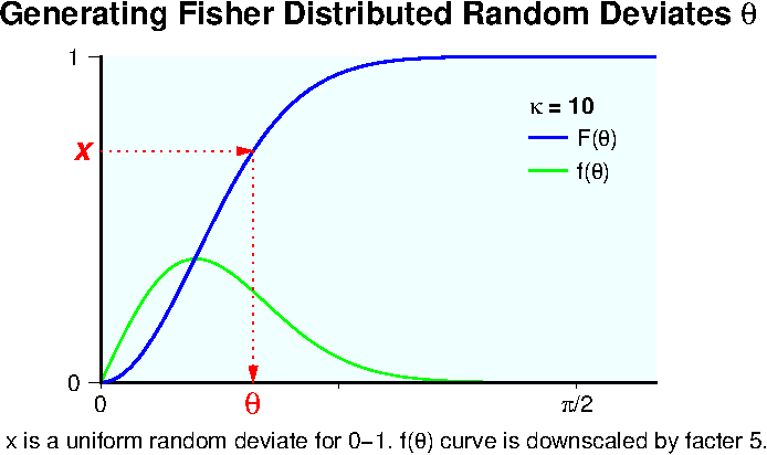
The probability \(f(\theta)d\theta\) of finding a vector between \(\theta\) and \(\theta + d\theta\) in the Fisher distribution is given by, \[ f(\theta)d\theta = \frac{\kappa}{2\sinh\kappa}e^{\kappa\cos\theta}\sin\theta d\theta. \] To create a random deviate \(\theta\) using a uniform random deviate \(x\) where \(x\) is between 0 and 1, the next relation should hold. \[ f(\theta)d\theta = dx, \] that is, \[ \frac{dx}{d\theta} = f(\theta). \] Solving this equation, \[ x = \int_0^\theta f(\theta)d\theta = F(\theta) = \frac{1}{2\sinh(\kappa)}(e^\kappa - e^{\kappa\cos\theta}), \] where \(F(\theta)\) is the cumulative distribution function of the probability density function \(f(\theta)\). Hence, the random deviate \(\theta\) is given by \(F^{-1}(x)\) which is the inverse function to \(F(\theta)\), as illustrated in the figure below.
Therefore, using the uniform random deviates \(x_1\) and \(x_2\) between 0 and 1, the random generator of Fisher distribution is given by the next equations together with the random deviate \(\varphi\). \begin{eqnarray} \theta & = & \arccos\left( 1 + {1 \over \kappa}\log\left(1 - (1 - e^{-2\kappa})x_1\right) \right), \label{eq09} \\ \varphi & = & 2\pi x_2. \label{eq10} \end{eqnarray}
However, program "tmeandir" uses another random generator for Fisher distribution which was developed by N.I. Fisher and others in 1981 (described at p.59 of Fisher et al. 1987). In this random generator, the equation for the random deviate \(\theta\) is given as below, and for \(\varphi\) it is the same as \eqref{eq10}. \begin{equation} \theta = 2\arcsin\sqrt{ \frac{-\log(x_1(1-e^{-2\kappa})+e^{-2\kappa})}{2\kappa} }. \label{eq11} \end{equation} Analytically, equation \eqref{eq11} is identical to \eqref{eq09} if \(x_1\) is replaced by \(1-x_1\) in \eqref{eq09}. Nevertheless, numerically \eqref{eq11} seems to be superior to \eqref{eq09} especially for small \(\kappa\). According to McFadden & McElhinny (1990), this generator gives the best performance. As for the uniform random deviate \(x\) between 0 and 1, program "tmeandir" uses function "ran1" of Press et al. (1992).
References:
- Fisher, N. I., T. Lewis, and B. J. J. Embleton, Statistical analysis of spherical data, 329 pp., Cambridge University Press, Cambridge, 1987.
- McFadden, P. L., and F. J. Lowes, The discrimination of mean directions drawn from Fisher distributions, Geophys. J. R. astr. Soc., 67, 19-33, 1981.
- McFadden, P. L., and M. W. McElhinny, Classification of the reversal test in palaeomagnetism, Geophys. J. Int., 103, 725-729, 1990.
- Press, W.H., S.A. Teukolsky, W.T. Vetterling, and B.P. Flannery, Numerical Recipes in C: The Art of Scientific Computing (Second Edition), 994 pp., Cambridge University Press, Cambridge, 1992.
- Watson, G. S., Analysis of dispersion on a sphere, Mon. Not. Roy. Astr. Soc. Geophys. Suppl., 7, 153-159, 1956.