 Statistical Tests: Test of distribution; histo & histo2
In any fields of science, it is often important to know whether a certain data is distributed as a known distribution such as the normal (Gauss) distribution. It is also often necessary to know whether the distributions of two data sets are different. Effective and easy way to solve these questions is to draw histograms of the data and carry out statistical tests, which are provided by programs "histo" and "histo2".
For such purposes, the null hypothesis would be like "H: the observed data are drawn from the population of the normal distribution", or "H: the two data sets are drawn from the same population distribution". It is stressed here that the statistical tests are aimed to disprove these null hypotheses. Hence, when the null hypotheses are not rejected, you cannot claim that the null hypotheses are true. You can only state that "the data is not inconsistent with the normal distribution", or "the two data distributions can be consistent with a single distribution".
Program "histo" tests whether a certain data set is distributed as a normal distribution or a log-normal distribution by using the Chi-square test and the Kolmogorov-Smirnov test. In the Chi-square test, the data is divided in bins so that the number of data in each bin is as equal as possible. For this purpose, bin boundaries are determined as each bin becomes equal fraction of the probability density of the normal (log-normal) distribution with the mean and standard deviation of the data. Chi-square test is repeated multiple times for bin numbers starting from four bins and stops when the data number of each bin expected from the supposed distribution becomes less than five.
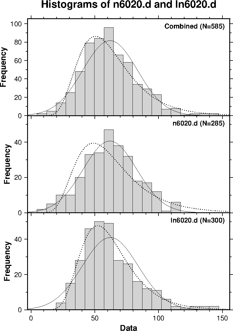
Program "histo2" reads two data files and tests whether the distributions of the two data sets are different by the Chi-square test and the Kolmogorov-Smirnov test. In the Chi-square test, bin boundaries are determined so that the cumulative distribution of the combined data is evenly divided. Similarly to "histo", the Chi-square test is repeated with different bin numbers. Program "histo2" also carries out the distribution test of normal/log-normal distribution to each data set. An example of histograms plotted by "histo2" is shown below in which artificial random data of normal and log-normal distributions are compared. Results of the statistical test are written to stdout (terminal display on Linux).
Chi-square test
The Chi-square test measures degrees of difference between the frequencies of the binned data and those of a known distribution. Let \(N_B\) is the number of bins of the histogram, the Chi-square statistic is given by, \begin{equation} \chi^2 = \sum_{i=1}^{N_B}\frac{(n_i - e_i)^2}{e_i}, \label{eq01} \end{equation} where \(n_i\) is the frequency of the data in the \(i\)'th bin and \(e_i\) is the expectation from a known distribution. It is known that the distribution of this statistic is well approximated by the \(\chi^2\) distribution with the degrees of freedom \(\nu=N_B-1\) when \(N_B\) ≥ 5 and \(e_i\) ≥ 5 (Hoel, 1971). If the observed \(\chi^2\) exceeds the critical value corresponding to the significance level \(\alpha\), we reject the null hypothesis that the data set is a sample from the known distribution. When the data distribution is tested against the normal or log-normal distributions which are determined from the mean and standard deviation of the observed data, the degrees of freedom is decreased by the number of parameters used. Hence, in such cases the degrees of freedom is \(\nu = N_B-3\).
The Chi-square test is also applied to test whether the distributions of two data sets are different. Let \(R_i\) and \(S_i\) be the data frequencies in the same \(i\)'th bin of the first and second data sets, respectively. The Chi-square statistic is given by, \begin{equation} \chi^2 = \sum_{i=1}^{N_B}\frac{(\sqrt{S/R}R_i - \sqrt{R/S}S_i)^2}{R_i + S_i}, \label{eq02} \end{equation} where \(R\) and \(S\) are the total data numbers of the first and second data sets, respectively (Press et al., 1992). The statistic of \eqref{eq02} is approximately distributed as the \(\chi^2\) distribution with the degrees of freedom \(\nu=N_B-1\).
Kolmogorov-Smirnov test
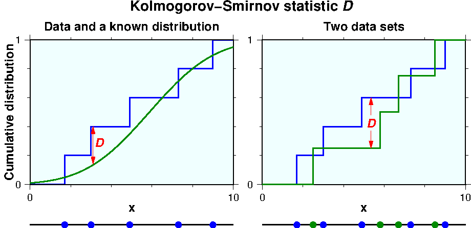
The Kolmogorov-Smirnov (K-S) test measures degrees of difference of the two cumulative distribution curves between the observed data and a known distribution or another data set. The larger the difference it would be more probable that the two distributions are different. Consider \(N\) data \(x_i (i=1 \cdots N)\) which are sorted in ascending order. In the K-S test, the cumulative distribution function of the data \(S_N(x)\) is given by the step function, \begin{equation} S_N(x) = \left\lbrace \begin{array}{cl} 0 & (x < x_1), \\ i/N & (x_i ≤ x < x_{i+1}), \label{eq03} \\ 1 & (x ≥ x_N). \end{array} \right. \end{equation} When one data distribution is compared to a known distribution, the K-S statistic is the maximum value of the absolute difference of the cumulative distribution curves \(S_N(x)\) of the data and \(F(x)\) of the known distribution, \begin{equation} D = \max_{-\infty< x <\infty} |S_N(x) - F(x)|. \label{eq04} \end{equation} To compare the distributions of two data sets, the K-S statistic \(D\) is given by, \begin{equation} D = \max_{-\infty< x <\infty} |S_{N_1}(x) - S_{N_2}(x)|, \label{eq05} \end{equation} where \(S_{N_1}(x)\) and \(S_{N_2}(x)\) are the cumulative distribution functions of the first and second data, respectively. The K-S statistic \(D\) is schematically illustrated in the next figures in which the observed data are compared to a known distribution (left) and to another data set (right).
Using the observed statistic \(D_{obs.}\), there are several ways to estimate the significance probability \(P\) which is the probability of obtaining the value of the test statistic if the null hypothesis is true (the null hypothesis is rejected if \(P\) is smaller than the given significance level \(\alpha\)). Here, following Press et al. (1992), let \(Q_{KS}\) be a function given by, \begin{equation} Q_{KS}(\lambda) = 2\sum_{j=1}^\infty (-1)^{j-1} e^{-2j^2\lambda^2}. \label{eq06} \end{equation} Using this function, \(P\) is approximately given by, \begin{equation} P(D>D_{obs.}) = Q_{KS}\left(\left[\sqrt{N_e} + 0.12 + 0.11\left/\sqrt{N_e}\right.\right]D_{obs.}\right), \label{eq07} \end{equation} where \(N_e\) is the effective number of data; \begin{equation} N_e = N, \label{eq08} \end{equation} for data and a known distribution of \eqref{eq04}, and \begin{equation} N_e = \frac{N_1 N_2}{N_1 + N_2}, \label{eq09} \end{equation} for two data sets of \eqref{eq05}. Although accuracy of equation \eqref{eq07} becomes higher for larger \(N_e\), it seems to be already quite good for the numbers as small as \(N_e \geq 4\) according to Press et al (1992). It should be mentioned, however, that this may not be true when data is compared to a normal (log-normal) distribution in programs "histo" and "histo2". This is because the programs use two parameters, mean and standard deviation, which are determined from the data. In such a case, Press et al. (1992) recommends to perform a simulation method, which "histo" and "histo2" do not include.
Download and installation of the program
Functions related to the normal, log-normal, and \(\chi^2\) distributions
In the followings, \(f(x)\) and \(F(x)\) are the probability density of \(x\) and its cumulative distribution, respectively. \(P(x_c)\) is the probability for \(x\) to exceeds a critical value \(x_c\). Definitions and notations are after Crow et al. (1960), Kohari (1973), and Press et al. (1992).
normal distribution:
\begin{equation} f(x) = {1 \over \sqrt{2\pi}\sigma}e^{-(x-\mu)^2/2\sigma^2}. \label{eq10} \end{equation} where \(\mu\) and \(\sigma^2\) are the mean and the variance of \(x\). Introducing the standardized variable, \begin{equation} z = (x - \mu)/\sigma, \label{eq11} \end{equation} the probability density of \(z\) is written as, \begin{equation} f(z) = {1 \over \sqrt{2\pi}}e^{-z^2/2}. \label{eq12} \end{equation} As the indefinite integral of \(f(z)\) is not expressed by elementary functions, it is difficult to show \(\int_{-\infty}^\infty f(z)=1\). However, intuitive derivation is given as the followings (may be mathematically not strict). Consider a double integral as, \[ \int_{-\infty}^\infty e^{-u^2/2}du \int_{-\infty}^\infty e^{-v^2/2}dv = \int_{-\infty}^\infty\int_{-\infty}^\infty e^{-(u^2 + v^2)/2}du dv. \] Introducing \(r\) and \(\theta\) as, \[ u = r\cos\theta, \quad v = r\sin\theta, \quad dudv = r dr d\theta, \] the double integral is determined as, \[ \int_0^{2\pi}d\theta\int_0^\infty r e^{-r^2/2}dr = 2\pi\left[-e^{-r^2/2}\right]_0^\infty = 2\pi. \] Hence, \(\int_{-\infty}^\infty e^{-z^2/2}dz=\sqrt{2\pi}\), i.e. \(\int_{-\infty}^\infty f(z)=1\).
Using \eqref{eq12}, the mean and variance of \(x\) are, \begin{eqnarray*} E[x] & = & {1 \over \sqrt{2\pi}\sigma}\int_{-\infty}^\infty x e^{-(x-\mu)^2/2\sigma^2}dx, \\ & = & {1 \over \sqrt{2\pi}}\int_{-\infty}^\infty(\sigma z + \mu) e^{-z^2/2}dz, \\ & = & {\sigma \over \sqrt{2\pi}}\left[-e^{-z^2/2}\right]_{-\infty}^\infty + {\mu \over \sqrt{2\pi}}\int_{-\infty}^\infty e^{-z^2/2}dz = \mu. \end{eqnarray*} \begin{eqnarray*} E[(x-\bar x)^2] & = & {1 \over \sqrt{2\pi}\sigma}\int_{-\infty}^\infty (x-\mu)^2 e^{-(x-\mu)^2/2\sigma^2}dx, \\ & = & {\sigma^2 \over \sqrt{2\pi}}\int_{-\infty}^\infty z^2 e^{-z^2/2}dz = {\sigma^2 \over \sqrt{2\pi}}\int_{-\infty}^\infty z\left(-e^{-z^2/2}\right)^{'} dz, \\ & = & {\sigma^2 \over \sqrt{2\pi}}\left[-ze^{-z^2/2}\right]_{-\infty}^\infty + {\sigma^2 \over \sqrt{2\pi}}\int_{-\infty}^\infty e^{-z^2/2}dz = \sigma^2. \end{eqnarray*} In the last line, partial integration was used and the first term was set to zero without a proof (\(\int_{-\infty}^\infty z^2 e^{-z^2/2}dz=\sqrt{2\pi}\) is also tabulated in the manual of mathematical formulas).
\(\def\erf{\mathop{\mathrm{erf}}\nolimits}\) \(\def\erfc{\mathop{\mathrm{erfc}}\nolimits}\) As \(\int_{-\infty}^x f(x)dx\) is not expressed by elementary functions, the error function \(\erf(x)\) and the complementary error function \(\erfc(x)\) are introduced to represent the cumulative distribution \(F(x)\); \begin{eqnarray} \erf(x) & = & {2 \over \sqrt{\pi}}\int_0^x e^{-t^2}dt, \label{eq13} \\ \erfc(x) & = & 1 - \erf(x) = {2 \over \sqrt{\pi}}\int_x^\infty e^{-t^2}dt, \label{eq14} \end{eqnarray} When \(z ≥ 0\), using \eqref{eq12} and introducing \(t=z/\sqrt{2}\), \begin{eqnarray*} F(z) & = & {1 \over \sqrt{2\pi}}\int_{-\infty}^z e^{-z^2/2} dz, \\ & = & 0.5 + {1 \over \sqrt{2\pi}}\int_0^z e^{-z^2/2} dz = 0.5 + {1 \over \sqrt{\pi}}\int_0^{z/\sqrt{2}} e^{-t^2} dt, \\ & = & 0.5 + {1 \over 2}\erf\left({z \over \sqrt{2}}\right). \end{eqnarray*} Similarly for \(z < 0\), \begin{eqnarray*} F(z) & = & 1 - {1 \over \sqrt{2\pi}}\int_z^\infty e^{-z^2/2} dz, \\ & = & 1 - {1 \over \sqrt{\pi}}\int_{z/\sqrt{2}}^\infty e^{-t^2} dt = 1 - {1 \over 2}\erfc\left({z \over \sqrt{2}}\right), \\ & = & 0.5 + {1 \over 2}\erf\left({z \over \sqrt{2}}\right). \end{eqnarray*} Summarizing the above results, for all range of \(z\) and \(x\), \begin{eqnarray} F(z) & = & 0.5 + {1 \over 2}\erf\left({z \over \sqrt{2}}\right), \label{eq15} \\ F(x) & = & 0.5 + {1 \over 2}\erf\left(\frac{x-\mu}{\sqrt{2}\sigma}\right). \label{eq16} \end{eqnarray}
The probability \(P(z_c)\) for \(z\) to exceed a critical value \(z_c\) is obtained by substituting \eqref{eq15} to \(P(z_c)= 1-F(z_c)\) (similarly for \(x\)), \begin{eqnarray} P(z_c) & = & {1 \over 2}\erfc\left({z_c \over \sqrt{2}}\right), \label{eq17} \\ P(x_c) & = & {1 \over 2}\erfc\left(\frac{x_c-\mu}{\sqrt{2}\sigma}\right). \label{eq18} \end{eqnarray}
log-normal distribution:
The log-normal distribution is the distribution of \(x\) when \(y=\log x\) is distributed as the normal distribution. Let \(g(y)\) be the probability density of \(y\), \begin{equation} g(y) = {1 \over \sqrt{2\pi}\sigma}e^{-(y-\mu)^2/2\sigma^2}, \label{eq19} \end{equation} where \begin{equation} y = \log x \quad (x > 0). \label{eq20} \end{equation} The probability density \(f(x)\) of \(x=e^y\) satisfies \[ g(y)dy = f(x)dx. \] Hence, \begin{eqnarray} f(x) & = & g(y){dy \over dx} = g(\log x){1 \over x}, \nonumber \\ & = & {1 \over \sqrt{2\pi}\sigma x}e^{-(\log x-\mu)^2/2\sigma^2} \quad (x > 0), \label{eq21} \end{eqnarray} and it is obvious that \(\int_0^\infty f(x) = 1\).
Mean of \(x\) is derived as the followings. \[ E[x] = \int_0^\infty xf(x)dx = {1 \over \sqrt{2\pi}\sigma}\int_0^\infty e^{-(\log x-\mu)^2/2\sigma^2}dx. \] Introducing \(t=\log x\), and hence, \(dx=e^t dt\), \begin{eqnarray} E[x] & = & {1 \over \sqrt{2\pi}\sigma}\int_{-\infty}^\infty e^{-(t-\mu)^2/2\sigma^2+t}dt, \nonumber \\ & = & e^{(2\mu+\sigma^2)/2}{1 \over \sqrt{2\pi}\sigma}\int_{-\infty}^\infty e^{-(t-(\mu+\sigma^2))^2/2\sigma^2}dt, \nonumber \\ & = & e^{\mu+\sigma^2/2}. \label{eq22} \end{eqnarray} To obtain the variance of \(x\), we first derive \(E[x^2]\). \begin{eqnarray*} E[x^2] & = & \int_0^\infty x^2f(x)dx = {1 \over \sqrt{2\pi}\sigma}\int_0^\infty x e^{-(\log x-\mu)^2/2\sigma^2}dx, \\ & = & {1 \over \sqrt{2\pi}\sigma}\int_{-\infty}^\infty e^{t-(t-\mu)^2/2\sigma^2+t}dt, \\ & = & e^{2(\mu+\sigma^2)}{1 \over \sqrt{2\pi}\sigma}\int_{-\infty}^\infty e^{-(t-(\mu+2\sigma^2))^2/2\sigma^2}dt, \\ & = & e^{2(\mu+\sigma^2)}. \end{eqnarray*} Hence, the variance of \(x\) is given by, \begin{eqnarray} E[(x-\bar x)^2] & = & E[x^2] - {\bar x}^2, \nonumber \\ & = & e^{2(\mu+\sigma^2)} - e^{2\mu+\sigma^2}, \nonumber \\ & = & e^{2\mu+\sigma^2}(e^{\sigma^2}-1). \label{eq23} \end{eqnarray}
The cumulative distribution function \(F(x)\) of the log-normal distribution is given by, \[ F(x) = {1 \over \sqrt{2\pi}\sigma}\int_0^x {1 \over x}e^{-(\log x-\mu)^2/2\sigma^2}dx. \] Introducing \(t=-(\log x-\mu)/\sqrt{2}\sigma\), and hence, \(dx=-\sqrt{2}\sigma x dt\), \begin{eqnarray} F(x) & = & -{1 \over \sqrt{\pi}}\int_\infty^{-(\log x-\mu)/\sqrt{2}\sigma}e^{-t^2}dt, \nonumber \\ & = & {1 \over \sqrt{\pi}}\int_{-(\log x-\mu)/\sqrt{2}\sigma}^\infty e^{-t^2}dt, \nonumber \\ & = & {1 \over 2}\erfc\left(-\frac{\log x-\mu}{\sqrt{2}\sigma}\right). \label{eq24} \end{eqnarray}
Probability \(P(x_c)=1-F(x_c)\) for \(x\) to exceed \(x_c\) is, \begin{equation} P(x_c) = 1 - {1 \over 2}\erfc\left(-\frac{\log x_c-\mu}{\sqrt{2}\sigma}\right) = 0.5 + {1 \over 2}\erf\left(-\frac{\log x_c-\mu}{\sqrt{2}\sigma}\right). \label{eq25} \end{equation}
\(\chi^2\) distribution:
\begin{equation} f(x) = \frac{1}{2^{\nu \over 2}\Gamma\left({\nu \over 2}\right)}x^{{\nu \over 2}-1}e^{-{x \over 2}} \quad (x > 0). \label{eq26} \end{equation} To derive the cumulative distribution \(F(x)\), we use the following incomplete gamma functions, \begin{eqnarray*} \gamma(a,x) & = & \int_0^x t^{a-1}e^{-t}dt, \\ \Gamma(a,x) & = & \int_x^\infty t^{a-1}e^{-t}dt = \Gamma(a) - \gamma(a,x). \end{eqnarray*} Integrating \eqref{eq26}, \[ F(x) = \frac{1}{2^{\nu \over 2}\Gamma\left({\nu \over 2}\right)}\int_0^x x^{{\nu \over 2}-1}e^{-{x \over 2}}dx. \] Introducing \(t=x/2\), and hence, \(dx=2dt\), \begin{eqnarray} F(x) & = & \frac{1}{2^{\nu \over 2}\Gamma\left({\nu \over 2}\right)}\int_0^t 2^{{\nu \over 2}-1}t^{{\nu \over 2}-1}e^{-t}2dt, \nonumber \\ & = & \frac{1}{\Gamma\left({\nu \over 2}\right)}\int_0^{x/2}t^{{\nu \over 2}-1}e^{-t}dt, \nonumber \\ & = & \frac{\gamma\left({\nu \over 2},{x \over 2}\right)}{\Gamma\left({\nu \over 2}\right)}. \label{eq27} \end{eqnarray} Similarly, \(P(x_c)=1-F(x_c)\) is given by, \begin{equation} P(x_c) = \frac{\Gamma\left({\nu \over 2},{x \over 2}\right)}{\Gamma\left({\nu \over 2}\right)}. \label{eq28} \end{equation}
References:
- Crow, E. L., F. A. Davis, and M. W. Maxfield, Statistics Manual, 288 pp., Dover Pub. Inc., New York, 1960.
- Hoel, P. G., Introduction to Mathematical Statistics, 409 pp., John Wiley & Sons, Inc., New York, 1971.
- Kohari, A., Introduction to Probability and Statistics, 300 pp., Iwanami Shoten Pub., Tokyo, 1973. (in Japanese)
- Press, W.H., S.A. Teukolsky, W.T. Vetterling, and B.P. Flannery, Numerical Recipes in C: The Art of Scientific Computing (Second Edition), 994 pp., Cambridge University Press, Cambridge, 1992.