 Statistical Tests: Test of a common mean; tmean
In the field of statistics, certain characteristics are measured from a limited number of data (called a sample) which are randomly drawn from a whole collection of data (called a population), and deduce a conclusion about the population based on the measurements of the sample. Hereafter, the mean, the standard deviation, and the variance of a sample are denoted by \(\bar x\), \(s\), and \(s\)\(^2\), respectively, and those of a population by \(\mu\), \(\sigma\), and \(\sigma\)\(^2\), respectively. In a statistical test, we use a theorem (proposition) that a certain quantity (called a statistic) calculated from the measurements of a sample is distributed as a certain known distribution. For instance, it is well known that a mean of \(n\) data drawn from a population of normal distribution, \(\bar x=\frac{1}{n}\sum_{i=1}^n x_i\), is distributed as a normal distribution with a mean \(\mu\) and a variance \(\sigma^2/n\). Even for this well known theorem, it is quite difficult to prove, as known from a statistics text book in which pages are spent for its demonstration. However, as a practical worker of statistical tests, it is easy to carry out the test if we simply believe the validity of the theorems.
Test of a common mean
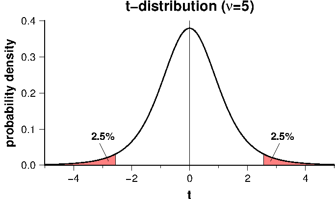
Program "tmean" tests whether two samples of scalar data share a common population mean. It uses Student's \(t\)-test when the population variances are equal and Welch's \(t\)-test when they are unequal. Let the data number, the mean, and the variance of sample 1 be denoted as \(n_1\), \(\bar x_1\), and \(s_1^2\), respectively, and those of sample 2 as \(n_2\), \(\bar x_2\), and \(s_2^2\). We assume the next null hypothesis, \begin{equation} \mu_1 - \mu_2 = 0. \nonumber \end{equation} Under the null hypothesis, when the population variances are equal (student's \(t\)-test), the following statistic \(t\) is distributed as a \(t\)-distribution with a degrees of freedom \(\nu = n_1 + n_2 - 2\), \begin{equation} t = \frac{\bar x_1 - \bar x_2}{s_p \sqrt{\frac{1}{n_1}+\frac{1}{n_2}}}, \label{eq01} \end{equation} where, \begin{equation} s_p^2 = \frac{s_1^2(n_1-1) + s_2^2(n_2-1)}{n_1 + n_2 - 2}, \label{eq02} \end{equation} is a pooled estimate of variance. When the population variances are unequal (Welch's \(t\)-test), the next statistic \(t\) is distributed as a \(t\)-distribution, \begin{equation} t = \frac{\bar x_1 - \bar x_2}{\sqrt{\frac{s_1^2}{n_1} + \frac{s_2^2}{n_2}}}, \label{eq03} \end{equation} with a number of degrees of freedom, \begin{equation} \nu = \frac{ \left(\frac{s_1^2}{n_1} + \frac{s_2^2}{n_2}\right)^2 }{ \frac{s_1^4}{n_1^2(n_1-1)} + \frac{s_2^4}{n_2^2(n_2-1)} }, \label{eq04} \end{equation} which is not necessarily an integer. To carry out the test, we calculate \(t\) from the observation by using \eqref{eq01} or \eqref{eq03}. Taking significance level \(\alpha\), if \(t\) is smaller than the lower \(\alpha/2\) point or larger than the upper \(\alpha/2\) point of the \(t\)-distribution curve (equal tails test), the null hypothesis is rejected and we conclude that the two population means are different. Figure below shows a typical \(t\)-distribution curve (\(\nu=5\)) in which rejection regions are indicated by red color for \(\alpha\)=5%.
Test of a common variance
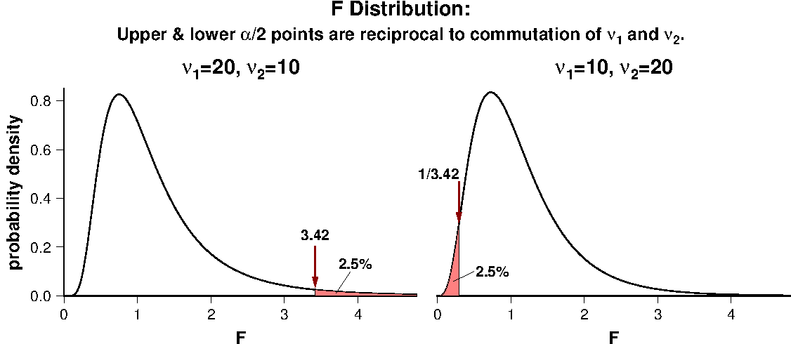
It is necessary to know whether the two populations share a common variance before performing the test of a common mean described above. For this purpose, we use a \(F\) test in which the next null hypothesis is assumed. \begin{equation} \frac{\sigma_1^2}{\sigma_2^2} = 1. \nonumber \end{equation} Under this null hypothesis, the ratio of the variances of two samples, \begin{equation} F = \frac{s_1^2}{s_2^2}, \label{eq05} \end{equation} is distributed as a \(F\) distribution with the degrees of freedom, \begin{equation} \nu_1 = n_1 - 1, \quad \nu_2 = n_2 - 1, \label{eq06} \end{equation} where \(n_1\) and \(n_2\) are numbers of the data contained in samples 1 and 2, respectively. If the statistic \(F\) obtained from the observation is larger or smaller than the upper or lower critical values corresponding to the specified significance level \(\alpha\), the null hypothesis is rejected. In practice, we take a larger variance as the numerator in \eqref{eq05} so that the calculated \(F\) is always larger than unity. If \(F\) is larger than the upper \(\alpha/2\) point, we reject the null hypothesis. Here, a cautionary note is given: in some books for practical statistical tests, it is erroneously stated that "as \(F\) is always lager than unity, upper \(\alpha\) point should be used in stead of \(\alpha/2\) point". This is incorrect because taking \(F\)>1 is only for convenience due to lack of the tables of percentage points for \(F\)<1 range. If relying on computation only, preprocessing of \(F\) is not necessary. Figure below shows that the lower 2.5% point (0.2925) of \(F\) distribution with \(\nu_1\)=10 and \(\nu_2\)=20 is the inverse of upper 2.5% point (3.4185) of \(F\) distribution with \(\nu_1\)=20 and \(\nu_2\)=10.
If the null hypothesis of a common population variance is rejected, we conclude that the two population variances are different and the Welch's \(t\)-test is used to test a common mean. Otherwise, Student's \(t\)-test is used. Here, an unavoidable problem arises in the latter case because we can say nothing about the difference of the variances when the null hypothesis is not rejected. We cannot claim that the two populations share a common variance. The reason of not rejected null hypothesis might be lack of large enough number of data or large errors contained in the means. Nevertheless, we proceed to the Student's \(t\)-test stating that the result of \(F\) test is not inconsistent with an equal variance. This situation is similar to the positive result of the reversals test in paleomagnetism.
Download and installation of the program
Summaries of functions related to \(t\)- and \(F\) distributions
In the following, \(f(x)\) is the probability density of \(x\) and \(P(x_c)\) is the probability for \(x\) to exceeds a critical value \(x_c\). Definitions and notations are after Crow et al. (1960), Kohari (1973), and Press et al. (1992).
\(t\)-distribution:
\begin{eqnarray} f(t) & = & \frac{\Gamma({\nu+1 \over 2})}{\sqrt{\nu}\Gamma({\nu \over 2})\Gamma({1 \over 2})}\left(1+{t^2 \over \nu}\right)^{-{\nu+1 \over 2}}, \nonumber \\ & = & \frac{1}{\sqrt{\nu}B({\nu \over 2},{1 \over 2})}\left(\frac{\nu}{\nu+t^2}\right)^{{\nu+1 \over 2}}, \label{eq07} \end{eqnarray} where \[ \Gamma(z) = \int_0^\infty u^{z-1}e^{-u} du, \] is the gamma function which is the factorial function when \(z\) is an integer; \(\Gamma(n+1)=n!\). It is also worth notice that \(\Gamma(1/2)=\sqrt{\pi}\). In equation \eqref{eq07}, \(B(\nu/2,1/2)\) is the beta function given by, \[ B(z,w) = B(w,z) = \int_0^1 u^{z-1}(1-u)^{w-1} du, \] which is related to the gamma function by \[ B(z,w) = \frac{\Gamma(z)\Gamma(w)}{\Gamma(z+w)}. \] Integrating \(f(t)\) given by \eqref{eq07}, \[ P(t) = \int_t^\infty f(t)dt = \frac{1}{\sqrt{\nu}B({\nu \over 2},{1 \over 2})}\int_t^\infty \left(\frac{\nu}{\nu+t^2}\right)^{{\nu+1 \over 2}}dt. \] Introducing, \[ z = \frac{\nu}{\nu+t^2}, \quad dt = -\frac{\sqrt{\nu}}{2}z^{-{3 \over 2}}(1-z)^{-{1 \over 2}}dz, \] \(P(t)\) is written as, \begin{eqnarray} P(t) & = & \frac{1}{2 B({\nu \over 2},{1 \over 2})}\int_0^{\nu \over \nu+t^2}z^{{\nu \over 2}-1}(1-z)^{{1 \over 2}-1}dz, \nonumber \\ & = & \frac{1}{2}I_{{\nu \over \nu+t^2}}\left({\nu \over 2},{1 \over 2}\right), \label{eq08} \end{eqnarray} where \[ I_x(a,b) = \frac{1}{B(a,b)}\int_0^x z^{a-1}(1-z)^{b-1} dz \quad (a,b > 0), \] is the incomplete beta function. To seek a \(t_c\) corresponding to a given \(P_c\), equation \eqref{eq08} is numerically solved by a root-finding routine "rtsafe" of Press et al. (1992) as \[ P_c - (1/2)I_{\nu/(\nu+t_c^2)}(\nu/2,1/2) = 0. \]
\(F\) distribution:
\begin{eqnarray} f(F) & = & \frac{\Gamma({\nu_1+\nu_2 \over 2})}{\Gamma({\nu_1 \over 2})\Gamma({\nu_2 \over 2})} \frac{\nu_1^{\nu_1 \over 2} \nu_2^{\nu_2 \over 2} F^{\nu_1-2 \over 2}}{(\nu_2+\nu_1 F)^{\nu_1+\nu_2 \over 2}} \quad (F > 0), \nonumber \\ & = & \frac{1}{B({\nu_1 \over 2},{\nu_2 \over 2})} \frac{\nu_1^{\nu_1 \over 2} \nu_2^{\nu_2 \over 2} F^{\nu_1-2 \over 2}}{(\nu_2+\nu_1 F)^{\nu_1+\nu_2 \over 2}} \quad (F > 0). \label{eq09} \end{eqnarray} Integrating this function, \[ P(F) = \int_F^\infty f(F)dF = \frac{1}{B({\nu_1 \over 2},{\nu_2 \over 2})} \int_F^\infty \frac{\nu_1^{\nu_1 \over 2} \nu_2^{\nu_2 \over 2} F^{\nu_1-2 \over 2}}{(\nu_2+\nu_1 F)^{\nu_1+\nu_2 \over 2}} dF. \] Introducing, \[ z = \frac{\nu_2}{\nu_2+\nu_1 F}, \quad dF = -\frac{\nu_2}{\nu_1}\frac{1}{z^2} dz, \] \(P(F)\) is written as, \begin{eqnarray} P(F) & = & \frac{1}{B({\nu_2 \over 2},{\nu_1 \over 2})} \int_0^{{\nu_2 \over \nu_2+\nu_1 F}}z^{{\nu_2 \over 2}-1}(1-z)^{{\nu_1 \over 2}-1} dz, \nonumber \\ & = & I_{\nu_2 \over \nu_2+\nu_1 F}\left({\nu_2 \over 2},{\nu_1 \over 2}\right). \label{eq10} \end{eqnarray} To seek a \(F_c\) corresponding to a given \(P_c\), equation \eqref{eq10} is numerically solved by a root-finding routine "rtsafe" of Press et al. (1992) as \[ P_c - I_{\nu_2/(\nu_2+\nu_1 F_c)}(\nu_2/2,\nu_1/2) = 0. \]
References:
- Crow, E. L., F. A. Davis, and M. W. Maxfield, Statistics Manual, 288 pp., Dover Pub. Inc., New York, 1960.
- Kohari, A., Introduction to Probability and Statistics, 300 pp., Iwanami Shoten Pub., Tokyo, 1973. (in Japanese)
- Press, W.H., S.A. Teukolsky, W.T. Vetterling, and B.P. Flannery, Numerical Recipes in C: The Art of Scientific Computing (Second Edition), 994 pp., Cambridge University Press, Cambridge, 1992.