ScatterMaker 6

Overview

Software for visualizing the distribution of data based on tabular datasets.

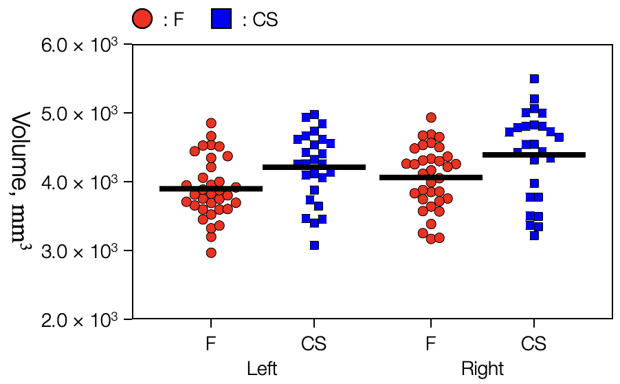
• Scatter plot for group comparisons

  

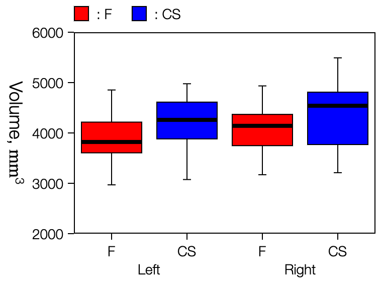
• Boxplot

  

• Scatter plot for examining correlations between two variables

  

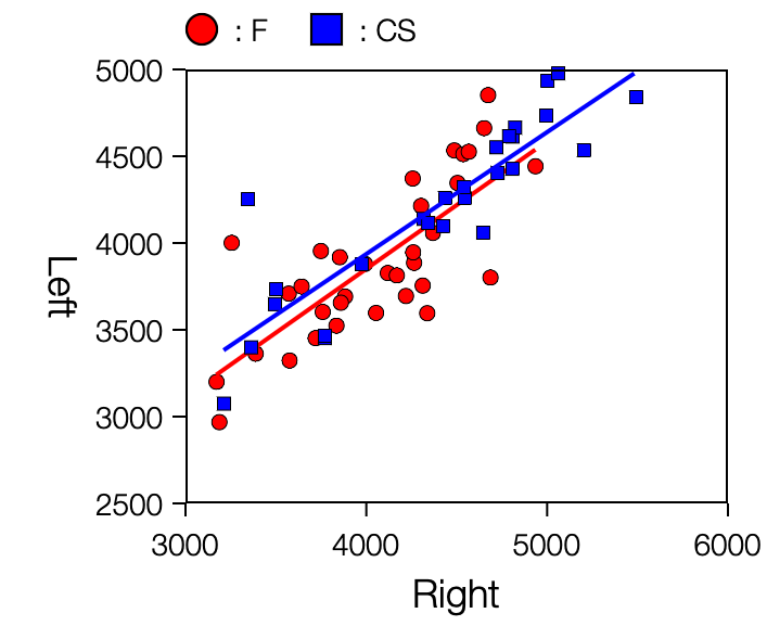
These three graph types allow users to visually explore the distribution and relationships within their data.

In scatter plots for group comparisons, the overlap of data points can be adjusted freely. The software automatically arranges points to produce an intuitive display with little or no overlap, making the underlying distribution easy to interpret.

In box plots, the box represents the median and the first and third quartiles, while the whiskers extend to the minimum and maximum values that are not considered outliers. Values lying more than 1.5 times the interquartile range (IQR) below the first quartile or above the third quartile are displayed as outliers.

In addition to descriptive statistics, the software provides basic statistical tests for objective evaluation of the data.

Each document contains a single data table together with multiple graph settings, allowing several visualizations to be managed within one file.

Table

• The first row must contain the column titles that identify the variables.
• Each column title must be unique.
• A table may contain columns used for grouping variables as well as columns containing measurement data.
• Grouping variables may contain either numeric or non-numeric values.

Creating a Table

• Import a CSV file.
• Import a tab-delimited text file.
• Paste data from another spreadsheet or table-based application.
• Enter data manually.

A table can be created using any of the four methods above.

Editing a Table

• Click (or tap) a cell to select it. Double-click (or double-tap) the cell to enter edit mode.
• Columns that are used in one or more graphs cannot be modified. All other columns can be edited by pasting data, entering values manually, or deleting rows or columns.

Exporting a Table

• Export to a file.
• Copy the table to the clipboard.

In both cases, the table is exported as tab-delimited text.

Graphs

• Three types of graphs can be created: scatter plots for group comparisons, box plots, and scatter plots for examining the correlation between two variables.
• There is no limit to the number of undo operations. However, the undo history is cleared when you switch to the table or another graph.
• Scatter plots for group comparisons and box plots can be converted to each other even after they have been created. In contrast, the graph type of a scatter plot used to examine the correlation between two variables cannot be changed after creation.

Creating a Graph

1. Switch the table to Variable Selection mode.
2. Select the variables to be used in the graph.
   • Scatter Plot (Group Comparison) and Box-and-Whisker Plot: Select one or more numeric variables.
   • Scatter Plot (Correlation): Select two numeric variables. The X- and Y-axes can be swapped after the graph is created.
   • Selecting a grouping variable is optional.

   

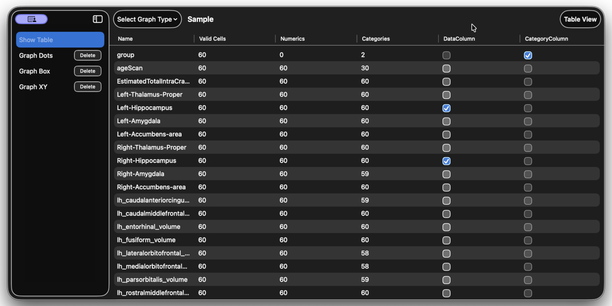
3. Select the graph type.
4. The graph is created.

Changing Graph Settings

• Select a graph to display it together with its settings.
• Settings are grouped by related functions.
  • Overall graph settings (colors, size, axes, etc.)
  • Settings for individual dots or boxes within the graph
  • Settings for the order and display names of variables
  • Value settings
• Settings can be changed individually by editing each item or updated in bulk by using copy and paste.

  When editing settings manually, some changes are applied immediately, while others take effect only after the Apply button is clicked.

  When using copy and paste, the software attempts to paste all copied settings. Any settings that are not applicable to the current graph, such as graph values, are automatically ignored.

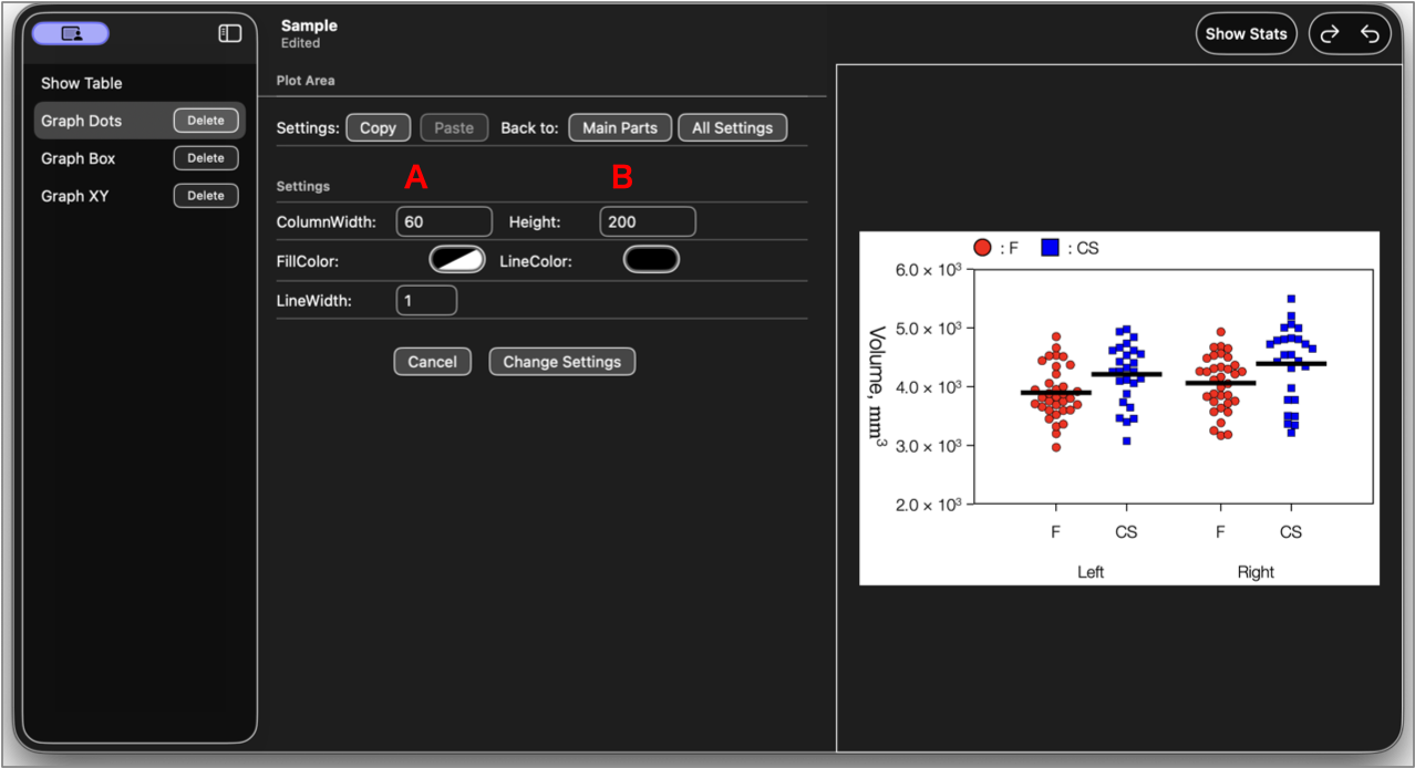
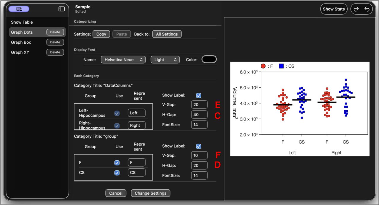
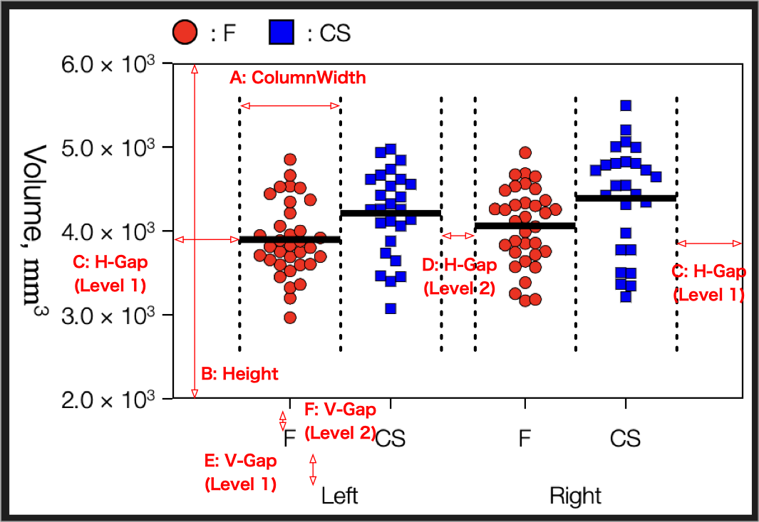
The main graph components are defined below.

Exporting Graphs

• Export an individual graph to a file.

  This option is available from the main graph settings screen after selecting a graph. Graphs are exported in PDF format.

• Copy an individual graph to the clipboard.

  The copied graph can be pasted into other applications that support PDF data.

• Export all graphs in the document as PDF files.

  Available on macOS only. This command can be accessed from the menu.

Important Settings

Graph Size

The overall graph size is determined automatically after the plot area size is specified (or calculated automatically) and other elements such as axes, titles, and legends are laid out according to the current settings. Because of this design, the overall graph size cannot be specified directly.

Plot Area Width

For correlation scatter plots, the width of the plot area is specified directly. For group comparison scatter plots and box-and-whisker plots, you specify the width of each group together with the gaps between category levels. The overall graph width is calculated from these values. Therefore, the total plot area width cannot be specified directly.

Data Point Size

Different marker shapes have different areas even when they have the same width. To prevent this from affecting the visual impression of the data distribution, ScatterMaker adjusts marker sizes so that all marker shapes have the same area.

You specify the approximate marker width. Since the marker areas are kept equal, the actual width varies slightly depending on the marker shape.

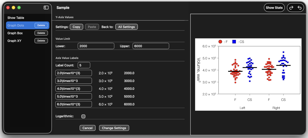
Axis Range and Tick Marks

The minimum axis value cannot be greater than the smallest data point, and the maximum axis value cannot be less than the largest data point.

Tick mark positions are calculated automatically when you enter their values.

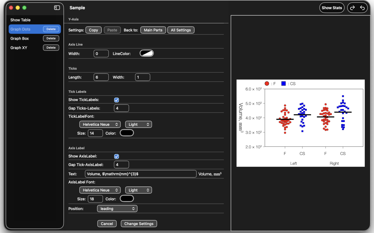
Axis labels and tick labels support a subset of TeX equation syntax. ScatterMaker does not fully implement TeX, but automatically converts common expressions such as fractions into inline notation.

For example, you can display 0.0015 as 1.5\times10^{-3}.

Axis Titles

Axis titles also support TeX-style notation. Text enclosed in $...$ is rendered using the same syntax supported for tick labels.

Descriptive Statistics and Between-Group Comparison Tests

Variance, Standard Deviation, Skewness, and Kurtosis

By default, “Use unbiased estimators...” is checked, and unbiased estimates are displayed. Unbiased estimators should be used when the data are obtained through random sampling from a population. In other words, unbiased estimators are appropriate in most cases.

Note: Strictly speaking, an unbiased estimator is not used for the standard deviation. To avoid confusion caused by differences among applications, the value shown is the square root of the unbiased estimator of variance, as used by many spreadsheet and statistical software packages.

Tests of Normality

The results of either the Shapiro-Wilk test¹⁾ or the Kolmogorov-Smirnov test²⁾ are displayed. The Shapiro-Wilk test is shown preferentially because it is considered to have greater statistical power³⁾, and because the Lilliefors correction for the Kolmogorov-Smirnov test is not implemented; consequently, the Kolmogorov-Smirnov test has particularly low power when the sample size is small³⁾. Due to limitations of the approximation method used, the Shapiro-Wilk test cannot be calculated for sample sizes greater than 5,000; in such cases, the result of the Kolmogorov-Smirnov test is displayed.

Tests of normality are displayed for reference only. As with other test results, the author cannot guarantee the accuracy of these results. Please interpret them at your own discretion. The approximation algorithms used are as follows:

1) Royston P: Approximating the Shapiro-Wilk W-test for non-normality. Statistics and Computing 1992: 2, 117-119.

2) Simard R, L'Ecuyer P: Computing the Two-Sided Kolmogorov-Smirnov Distribution. Journal of Statistical Software 2011: 39, 11.

3) Razali MN: Power comparisons of Shapiro-Wilk, Kolmogorov-Smirnov, Lilliefors and Anderson-Darling tests. Journal of Statistical Modeling and Analytics 2011: 2, 21-33.

Compatibility with Previous Versions

• The software attempts to open files created with previous versions on macOS only.
• Whenever possible, PDF data stored in the file is loaded.
• If the PDF created by a previous version is successfully loaded, an export button becomes available.
• Only some previous versions can be fully converted.
• Because the way graph data is handled has changed significantly in the new version, some settings, such as dot positioning, colors, and fonts, may not be reproduced exactly.
• The syntax for formulas has also been modified slightly, so some formulas may not be reproduced correctly. If a value cannot be restored, it is automatically replaced with its default value.
• Once a file created with a previous version has been opened and modified, it is saved in the new file format and can no longer be opened with the previous version.